Introduction to Null Steering

Sidelobe Canceller

Because the interference often arrive from sidelobes, null steering is closely related to a sidelobe canceller. The basic concept of a sidelobe canceller is straightforward. If the interference direction is known, one can always form a beam towards that direction, scale the beam to match the sidelobe gain of the original pattern, which is often referred to as the quiescent pattern, and subtract the scaled beam from the quiescent pattern to produce a null in that direction. Assume the interference is coming from 35 degrees in azimuth.

% define the quiescent steering weights
w_d = steervec(antpos,ang_d);

% define the interference direction and corresponding weights to steer
% array towards that direction
ang_i = 35;
w_i = steervec(antpos,ang_i);

To compute the gain of the quiescent pattern towards the interference direction, project the desired steering vector onto the interference direction. Then the gain is normalized by the pattern towards the interference direction so that when the scaled interference steering vector is subtracted from the desired steering vector, a null is formed towards the interference direction.

% compute the gain of the quiescent pattern towards the interference
% direction
g = w_d'*w_i/(w_i'*w_i);

% subtract the interference from the quiescent pattern
w_null = w_d - g'*w_i;

% examine patterns
ang_plot = -90:90;
P_d = mag2db(abs(arrayfactor(antpos,ang_plot,w_d)));
P_i = mag2db(abs(arrayfactor(antpos,ang_plot,g*w_i)));
P_null = mag2db(abs(arrayfactor(antpos,ang_plot,w_null)));

% plot the patterns
clf;
plot(ang_plot,[P_d(:) P_i(:) P_null(:)]);
hold on;
ylim([-40 20]);
plot([35 35],[-40 20],'r--');
hold off;
xlabel('Angles (degrees)');
ylabel('Power Pattern (dB)');
legend('Quiescent Pattern','Scaled Pattern to Interference','Nulled Pattern',...
    'Intereference Direction','Location','southwest');

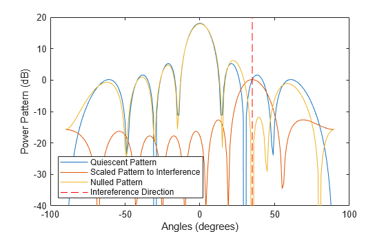
The dotted line marks the interference direction. It clearly shows that the sidelobe canceller creates a deep null formed at that direction.

Nulling through Space Projection

It might be tempting to extend this approach to multiple interferences. It seems that by cancelling out the sidelobe interferences one by one, all interferences can be removed from the resulting radiation pattern. This procedure is shown below.

% define the interference directions and compute nulling weights
ang_i = [-40 35 62];
w_i = steervec(antpos,ang_i);
w_null = w_d;

% following the aforementioned method, removing intererences one by one
for m = 1:numel(ang_i)
    g = w_d'*w_i(:,m)/(w_i(:,m)'*w_i(:,m));
    w_null = w_null - g'*w_i(:,m);
end
P_null = mag2db(abs(arrayfactor(antpos,ang_plot,w_null)));

% plot the patterns
clf;
plot(ang_plot,[P_d(:) P_null(:)]);
hold on;
ylim([-40 20]);
plot([ang_i;ang_i],repmat([-40;20],1,numel(ang_i)),'r--');
hold off;
xlabel('Angles (degrees)');
ylabel('Power Pattern (dB)');
legend('Quiescent Pattern','Nulled Pattern','Interference Directions','Location','southwest');

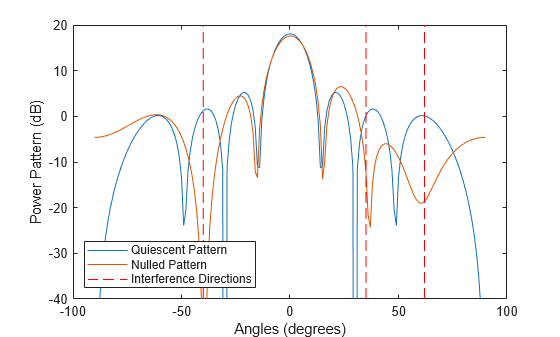
From the figure, the result is not very good. The interference on the left is suppressed well while the interferences on the right are not. This might be a bit of a surprise at first, but it is not hard to explain. When removing the interferences one by one, there is no consideration to make sure that when removing a later interference, the earlier interferences are still adequately suppressed. Therefore, this approach does not work well in practice for multiple interferences.

To accommodate multiple interferences, it is better to consider the nulling from a vector space perspective. In this approach, all interference directions form an interference subspace. Then the quiescent weights are projected to a subspace that is orthogonal to the interference subspace, ensuring that all interference are nulled out in the resulting pattern. This approach is shown in the following code snippet, using the nullweights function

% compute nulling weights
wn = nullweights(antpos,ang_d,ang_i);
P_null = mag2db(abs(arrayfactor(antpos,ang_plot,wn)));

% plot the patterns
clf;
plot(ang_plot,[P_d(:) P_null(:)]);
hold on;
ylim([-40 20]);
plot([ang_i;ang_i],repmat([-40;20],1,numel(ang_i)),'r--');
hold off;
xlabel('Angles (degrees)');
ylabel('Power Pattern (dB)');
legend('Quiescent Pattern','Nulled Pattern','Interference Directions','Location','southwest');

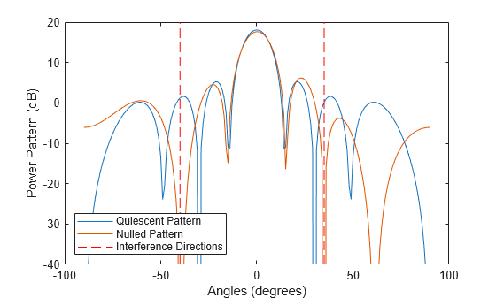
Note that deep nulls are formed on all interference directions.

The approach can be easily extended to a planar array. Next, the same approach is applied to a uniform rectangular array. The previous portion defines the array with a distance normalized to the wavelength. It is easy to use but is limited to a single frequency. The next snippet defines the array with absolute distance. This syntax can also accommodate a non-isotropic element.

% define the 4x4, half-wavelength rectangular array
N_rect = 4;
c = 3e8;
fc = 1e9;
lambda = freq2wavelen(fc,c);
d = lambda/2;
antrect = phased.URA(N_rect,d,'Element',phased.CosineAntennaElement);

% desired steering direction and nulling directions
ang_d_rect = [20;20];
ang_i_rect = [40 -30 -50;10 -10 5];

To use the nullweights function, the element position is extracted and normalized by the wavelength.

% compute nulling weights
wn = nullweights(getElementPosition(antrect)/lambda,ang_d_rect,ang_i_rect);

% plot the pattern
clf;
pattern(antrect,fc,'Type','powerdb','CoordinateSystem','rectangular','Weights',wn);
view(0,90);
hold on;
h = plot(ang_i_rect(1,:),ang_i_rect(2,:),'ro');
h.MarkerSize = 20;
hmb = plot(ang_d_rect(1,:),ang_d_rect(2,:),'b+');
hmb.MarkerSize = 20;
hold off

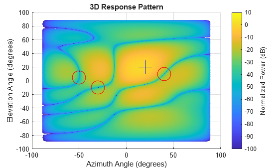
The nulls are successfully achieved at desired interference directions, as marked by the red circles. The main direction is marked by the blue cross.

Beam space null steering

Up to now, this example has focused on computing nulling weights in the element space, which means the computed weights are directly applied at each element. This approach fits the modern phased array workflow naturally as modern digital phased arrays enable magnitude and phase control at each array element. This provides the maximum flexibility. On the other hand, it is also the most expensive as each individual channel will require corresponding RF chain to operate.

To reduce the complexity, many deployed systems may take a hybrid approach. For example, many large phased arrays use subarray structures, where elements are grouped together to perform analog beamforming towards directions of interest first, and the results of these beamformed signals are then combined using digital weights to achieve the final beam pattern. Such systems are also sometimes referred to as switched beam systems or multibeam systems. To illustrate this idea, consider a 64-element half-wavelength uniform linear array. Assume the system only needs to look at a region from -30 to 30 degrees azimuth. Using analog beamformers, it generates 12 beams simultaneously to cover this area. The beams are shown in the following figure.

% define linear array element positions
Nlarge = 32;
antlargepos = (0:Nlarge-1)*0.5;

% form 8 beams within -30 to 30 degrees
N_beam = 12;
w_beam = steervec(antlargepos,asind((0:N_beam-1)/N_beam-1/2));
ang_beam_plot = -40:40;
antlargebeams = arrayfactor(antlargepos,ang_beam_plot,w_beam);
P_beams_plot = mag2db(abs(antlargebeams));

% plot beams
clf;
plot(ang_beam_plot,P_beams_plot);
xlabel('Angles (degree)');ylabel('Power (dB)');
ylim([-40 40]); grid on;

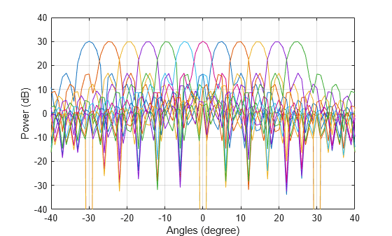
Note that downstream processing can only access the measurements from these 12 beams, thus the term "beam space". However, compared to the element space, the system now only needs to deal with 12 measurements instead of 32 measurements. This makes a huge difference in algorithm complexity. Coming back to the current example, without loss of generality, set the desired beam to be the center beam.

w_beam_d = zeros(N_beam,1);
w_beam_d(7) = 1;   % The center beam towards 0 azimuth

The interference directions are set to be -25, -15, and 9 degrees azimuth.

ang_beam_i = [-25 -15 9];

The corresponding responses toward interference directions are computed for each beam. These responses form the constraints subspace used in the slcweights to compute the nulling weights in the beam space.

beam_i_idx = ang_beam_i-ang_beam_plot(1)+1;
beam_constraints = antlargebeams(:,beam_i_idx);

% compute the nulling weights
w_beam_nulling = slcweights(w_beam_d,beam_constraints);
P_beams_nulling = w_beam_nulling'*antlargebeams;

% plot pattern
P_beams_nulling_plot = mag2db(abs(P_beams_nulling));
clf;
hold on;
plot(ang_beam_plot,P_beams_nulling_plot);
plot([ang_beam_i;ang_beam_i],repmat([-40;40],1,numel(ang_beam_i)),'r--');
hold off;
xlabel('Angles (degree)');ylabel('Power (dB)');
ylim([-40 40]); grid on;

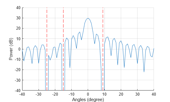
The figure shows that the nulls are successfully generated using existing beams.

Summary

This example explains the basic concept of nulling and shows how to achieve nulling in the beam pattern using Phased Array System Toolbox. The example also covers the nulling in both element space and beam space.

References

[1] Harry L. Van Trees, Optimum Array Processing, Wiley-Interscience, 2002