Range Estimation Using Stretch Processing

Introduction

Linear FM waveform is a popular choice in modern radar systems because it can achieve high range resolution by sweeping through a wide bandwidth. However, when the bandwidth is on the order of hundreds of megahertz, or even gigahertz, it becomes difficult to perform matched filtering or pulse compression in the digital domain because high-quality A/D converters are hard to find at such data rates.

Stretch processing, sometimes also referred to as deramp, is a technique that can be used in such situations. Stretch processing is performed in the analog domain.

The received signal is first mixed with a replica of the transmitted pulse. Note that the replica matches the return from the reference range. Once mixed, the resulting signal contains a frequency component that corresponds to the range offset measured from this reference range. Hence, the exact range can be estimated by performing a spectral analysis on the signal at the output of the mixer.

In addition, instead of processing the entire range span covered by the pulse, the processing focuses on a small window around a predefined reference range. Because of the limited range span, the output data of the stretch processor can be sampled at a lower rate, relaxing the bandwidth requirement for A/D converters

The following sections show an example of range estimation using stretch processing.

Simulation Setup

The radar system in this example uses a linear FM waveform with a 3 MHz sweeping bandwidth. The waveform can be used to achieve a range resolution of 50 m and a maximum unambiguous range of 8 km. The sample rate is set to 6 MHz, i.e., twice the sweeping bandwidth. For more information about the radar system, see Waveform Design to Improve Range Performance of an Existing System.

Three targets are located at 2000.66, 6532.63, and 6845.04 meters from the radar, respectively. Ten pulses are simulated at the receiver. These pulses contain echoes from the targets.

[rx_pulses, waveform] = helperStretchSimulate;
fs = waveform.SampleRate;

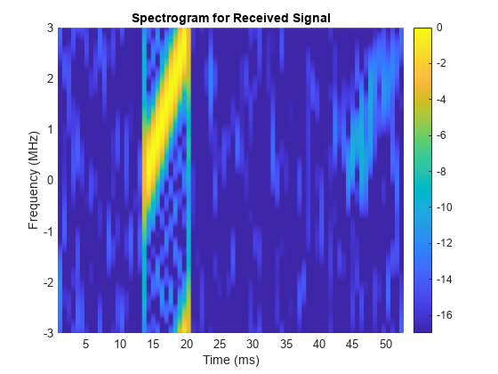
A time frequency plot of the received pulse is shown below. A coherent pulse integration is done before the plot to improve the signal-to-noise ratio (SNR). In the figure, the return from the first target can be clearly seen between 14 and 21 ms while the return from the second and third targets are much weaker, appearing after 45 ms.

helperStretchSignalSpectrogram(pulsint(rx_pulses,'coherent'),fs,...
    8,4,'Received Signal');

Stretch Processing

To perform stretch processing, first determine a reference range. In this example, the goal is to search targets around 6700 m away from the radar, in a 500-meter window. A stretch processor can be formed using the waveform, the desired reference range and the range span.

refrng = 6700;
rngspan = 500;
prop_speed = physconst('lightspeed');
stretchproc = getStretchProcessor(waveform,refrng,rngspan,prop_speed)

stretchproc = 
  phased.StretchProcessor with properties:

          SampleRate: 5.9958e+06
          PulseWidth: 6.6713e-06
           PRFSource: 'Property'
                 PRF: 1.8737e+04
          SweepSlope: 4.4938e+11
       SweepInterval: 'Positive'
    PropagationSpeed: 299792458
      ReferenceRange: 6700
           RangeSpan: 500

Next, pass the received pulses through the stretch processor.

y_stretch = stretchproc(rx_pulses);

Now, coherently integrate the pulses to improve the SNR.

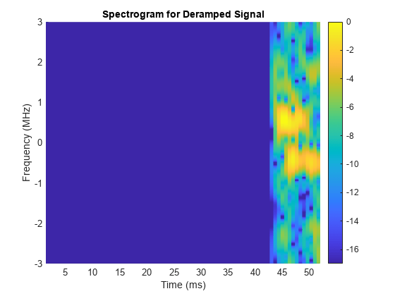
y = pulsint(y_stretch,'coherent');

The spectrogram of the signal after stretch processing is shown below. Note that the second and third target echoes no longer appear as a ramp in the plot. Instead, their time-frequency signatures appear at constant frequencies, around 0.5 and -0.5 MHz. Hence, the signal is deramped. In addition, there is no return present from the first target. In fact, any signal outside the ranges of interest has been suppressed. This is because the stretch processor only allows target returns within the range window to pass. This process is often referred to as range gating in a real system.

helperStretchSignalSpectrogram(y,fs,16,12,'Deramped Signal');

Range Estimation

To estimate the target range, plot the spectrum of the signal.

periodogram(y,[],2048,stretchproc.SampleRate,'centered');

From the figure, it is clear that there are two dominant frequency components in the deramped signal, which correspond to two targets. The frequencies of these peaks can be used to determine the true range values of these targets.

[p, f] = periodogram(y,[],2048,stretchproc.SampleRate,'centered');


[~,rngidx] = findpeaks(pow2db(p/max(p)),'MinPeakHeight',-5);
rngfreq = f(rngidx);
re = stretchfreq2rng(rngfreq,...
    stretchproc.SweepSlope,stretchproc.ReferenceRange,prop_speed)

re = 2×1
103 ×

    6.8514
    6.5174

The estimated ranges are 6518 and 6852 meters, matching the true ranges of 6533 and 6845 meters.

Reduced Sample Rate

As mentioned in the introduction section, an attractive feature of stretch processing is that it reduces the bandwidth requirement for successive processing stages. In this example, the range span of interest is 500 meters. The required bandwidth for the successive processing stages can be computed as

rngspan_bw = ...
    2*rngspan/prop_speed*waveform.SweepBandwidth/waveform.PulseWidth

rngspan_bw = 
1.4990e+06

Following the same design rule as in the original system, where twice the bandwidth is used as the sampling frequency, the new required sampling frequency becomes

fs_required = 2*rngspan_bw

fs_required = 
2.9979e+06

dec_factor = round(fs/fs_required)

dec_factor = 
2

The resulting decimator factor is 2. This means that after performing stretch processing in the analog domain, signals can be sampled at only half of the sampling frequency compared to the case where the stretch processing is not used. Thus, the requirement on the A/D converter has been relaxed.

To verify this benefit in simulation, the next section shows that the same ranges can be estimated with the signal decimated after stretch processing.

% Design a decimation filter
decimator = design(fdesign.decimator(dec_factor,'lowpass',...
    'N,F3dB',10,1/dec_factor),'SystemObject',true);

% Decimate
y_stretch = decimator(y_stretch);

This time, the power spectral density is plotted against ranges.

y = pulsint(y_stretch,'coherent');
[p, f] = periodogram(y,[],2048,fs_required,'centered');
rng_bin = stretchfreq2rng(f,...
    stretchproc.SweepSlope,stretchproc.ReferenceRange,prop_speed);
plot(rng_bin,pow2db(p));
xlabel('Range (m)'); ylabel('Power/frequency (dB/Hz)'); grid on;
title('Periodogram Power Spectral Density Estimate');

[~,rngidx] = findpeaks(pow2db(p/max(p)),'MinPeakHeight',-5);
re = rng_bin(rngidx)

re = 2×1
103 ×

    6.8504
    6.5232

The true range values are 6533 and 6845 meters. Without decimation, the range estimates are 6518 and 6852 meters. With decimation, the range estimates are 6523 and 6851 meters. Therefore, the range estimation yields the same result with roughly only half of the computations compared to the nondecimated case.

Summary

This example shows how to use stretch processing to estimate the target range when a linear FM waveform is used. It also shows that stretch processing reduces the bandwidth requirement.

Reference

[1] Mark Richards, Fundamentals of Radar Signal Processing, McGraw-Hill, 2005.