Spectrum Sharing Using Spectrum Sensing and Waveform Notching

This example uses:

This example illustrates the implementation and analysis of a technique for reducing mutual interference between non-cooperative radar and communication systems by inserting notches into the transmitted radar waveform. The frequency spectrum is analyzed by the radar system to determine regions occupied by a communications waveform, and a notched radar waveform that minimizes the power contained in those occupied regions is generated. This type of spectrum sharing approach enables coexistence of radar and communications systems operating in the same region of the frequency spectrum.

Introduction

Coexistence between radar and communications systems continues to be an active area of research as the frequency spectrums that these systems operate in become more crowded, particularly with the proliferation of 5G communications networks. Non-cooperative coexistence is an approach in which a radar and communication system are operating in the same frequency spectrum independently of one another and without any data exchange between systems.

The coexistence strategy explored in this example involves a radar and communications system operating in the same frequency band (a 100 MHz band around 3.5 GHz). The spectrum sharing behavior is realized by a cognitive radar system that adapts its waveform to avoid spectral overlap with the communications signal. The communications system operates freely and does not vary its transmission scheme based on the presence of the radar. Meanwhile, the radar detects the spectral location of the communications signal and inserts frequency nulls (referred to as "notches") into its transmit waveform, thereby reducing the mutual interference between the systems.

In this example, we focus on the signal level implementation of a spectrum sensing and waveform generation technique that make up the basis for this proposed coexistence strategy. Specifically, we implement the following two step process for generating a radar waveform with notches in the portion of the frequency spectrum occupied by the communications signal [1]:

Determine the optimal frequency region for radar waveform transmission in the presence of an Orthogonal Frequency-Division Multiplexing (OFDM) communications waveform based on a Fast Spectrum Sensing (FSS) algorithm [2].
Create and analyze a Pseudo-Random Optimized Frequency Modulation (PRO-FM) pulsed waveform with notches (areas of reduced spectrum power) in the region occupied by the communications waveform [3].

Once the process for spectrum sensing and waveform generation is examined, a simulation is run to determine the performance benefit of using a notched radar waveform in the presence of a communications signal.

Spectrum Sensing

In the coexistence scheme described in this example, a radar system minimizes the impact that its transmit waveform has on a communication system while simultaneously improving radar performance by notching the radar transmit waveform. In order for such a coexistence scheme to be effective, the radar system must continuously and quickly (on the order of a pulse repetition interval) determine an unoccupied region of the spectrum for transmission.

A popular FSS algorithm is implemented in this example [2]. This approach groups the spectrum into regions of high and low power interference plus noise, and then selects the transmit region by maximizing an objective function that balances the trade-off between the total bandwidth of the radar waveform with the anticipated Signal to Interference plus Noise Ratio (SINR) based on measurements of the spectrum that contains a communication waveform.

Generate Communications Signal

The communications signal occupying the frequency spectrum is made up of two non-overlapping OFDM transmissions. Each of these OFDM transmissions contains four carriers separated by 1 MHz (occupying a total of 4 MHz of bandwidth).

fc = 3.5e9;                            % Communications center frequency
separationFrequency = 1e6;             % 1 MHz carrier separation frequency
numCarriers = 4;                       % 4 carriers with 1 MHz separation
ofdmLocations = [fc-25e6;fc+25e6];     % One OFDM transmission at center frequency - 25 MHz, one at center frequency + 25 MHz
sampleRate = 200e6;                    % 200 MHz sample rate
numSamples = 400;                      % Collect 400 communications samples

% Helper used to generate communications signal
commsSignal = helperGenerateCommunicationsSignal(sampleRate,numCarriers,numSamples,separationFrequency,ofdmLocations,fc);

Once the communications signal has been generated, calculate and plot its power spectrum.

% Get the communications signal power spectrum
pComms = pspectrum(commsSignal,sampleRate);
pCommsDb = pow2db(pComms);

% Get the frequency samples of communications spectrum
fComms = helperSpectrumFrequencies(sampleRate,numel(pComms));

% Plot the power spectrum of the communications signal
plot(fComms/10^6,pCommsDb,'LineWidth',1);
xlabel('Frequency (MHz)'); ylabel('Power Spectrum (dB)');
title('Power Spectrum of Communications Signal');

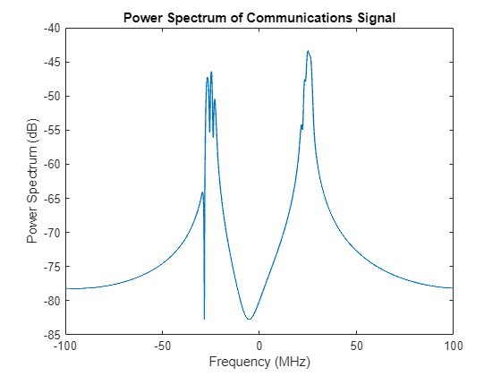
Figure contains an axes object. The axes object with title Power Spectrum of Communications Signal, xlabel Frequency (MHz), ylabel Power Spectrum (dB) contains an object of type line.

The power spectrum of the communications signal shows two occupied frequency bands. The ideal radar waveform in the coexistence scheme described in this example would contain very little power in the regions of the frequency spectrum where the communications signals are transmitted.

Separate Spectrum into High and Low Power Meso-Bands

The first step in the FSS algorithm is to divide the spectrum into high and low power interference plus noise regions. These regions are referred to as "meso-bands". No noise is added in this example, so in this case the spectrum power is solely due to the presence of the communications signal. The algorithm for splitting the spectrum into high and low power meso-bands is:

Create an alternating set of high and low power interference plus noise regions called meso-bands by comparing each sample to a user specified power threshold.
For each low power region, check if it is narrower than a user specified minimum meso-band bandwidth. If a low power region has a width lower than the user specified value, merge it with the adjacent high power bands.

First, set up the power threshold and minimum bandwidth based on the values used in [1].

pCommsDbMax = max(pCommsDb);     % Get the maximum communications signal power level
pThresholdDb = pCommsDbMax-15;   % User specified power threshold is set to be 15 dB below the max communications signal level
minBandwidth = 4e6;              % Minimum meso-band bandwidth is set to be 4 MHz

A helper function is used to separate the spectrum into high and low power meso-bands using the algorithm described above.

mesoBands = helperMesoBands(pComms,pThresholdDb,minBandwidth,sampleRate);

A plot of meso-bands shows that the frequency spectrum is separated into only 5 high and low power bands. This reduces the computational complexity of determining the optimal transmission region. Grouping the frequency spectrum into high and low power meso-bands using the user specified power threshold and minimum bandwidth heuristics is what makes this spectrum sensing algorithm computationally efficient.

a = helperPlotMesoBands(pComms,mesoBands,pThresholdDb,fComms,"Merged Meso-Bands",[-50 50]);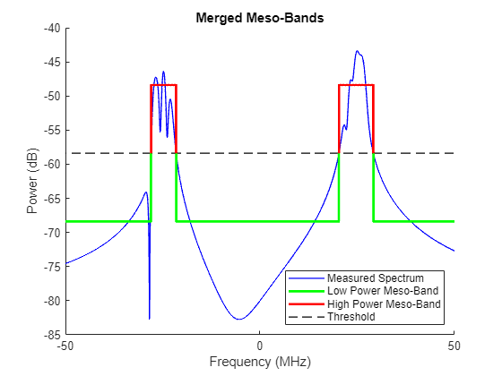

Figure contains an axes object. The axes object with title Merged Meso-Bands, xlabel Frequency (MHz), ylabel Power (dB) contains 7 objects of type line. These objects represent Threshold, Measured Spectrum, Low Power Meso-Band, High Power Meso-Band.

Select Meso-Band Combination that Maximizes Objective Function

The goal of this spectrum sensing algorithm is to transmit in the frequency range that maximizes the following objective function [2]:

$Objective = α * \overline{SINR} + (1 - α) * \overline{Bandwidth}$

where $\overline{SINR}$ and $\overline{Bandwidth}$ are the normalized SINR and bandwidth, and $α$ is a user specified weighting term that balances the tradeoff between increased bandwidth and increased SINR. The following equation is used to calculate SINR for a combination of meso-bands:

$SINR = \frac{τ * P_{s}}{P_{IN}}$

where $τ$ is the pulse width as a fraction of the pulse repetition interval, $P_{s}$ is the received signal power in a given meso-band based on the desired spectrum, and $P_{IN}$ is the received interference plus noise power in one pulse width in a given meso-band.

This objective function is calculated for every meso-band combination, and the combination that maximizes the objective function is selected as the radar waveform transmission region. In this case, there are only 5 meso-bands, so there are only $2^{5}$ -1=31 combinations of bands to calculate the objective value for.

For the purposes of this example, assume that the received radar signal power is 20 dB below the peak of the received communications signal power, the radar waveform pulse width is 5% of the pulse repetition interval (PRI), and the alpha value is set to 0.5.

peakSinrDb = -20;     % SINR of peak communications signal power vs. peak radar signal power
tau = 0.05;           % Pulse width as a fraction of pulse repitition interval
alpha = 0.5;          % Weighting factor between SINR and bandwidth

In order to determine the optimal transmission region, the desired waveform spectrum power is assumed to have a Gaussian shape. This spectral shape is desirable for radar waveforms because it results in low range sidelobes. This power spectrum is scaled to maintain the specified SINR.

% The desired waveform spectrum power has a Gaussian shape.
pWaveform = gausswin(numSamples);
pWaveformDb = pow2db(pWaveform);

% Scale the spectrum power for desired SINR
pWaveformScaledDb = pWaveformDb + (pCommsDbMax-max(pWaveformDb)) + peakSinrDb;
pWaveformScaled = db2pow(pWaveformScaledDb);

Plot the Gaussian radar waveform spectrum power along with the communications signal spectrum power used to calculate the objective function for all meso-band combinations.

% Plot the communications signal spectrum power along with the desired radar waveform
% spectrum power
helperPlotCommsWithRadarSpectrum(pComms,pWaveformScaled,'Full Radar Waveform',sampleRate,'Radar Waveform and Communications Signal Spectrum');

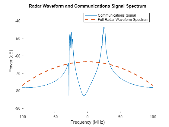
Figure contains an axes object. The axes object with title Radar Waveform and Communications Signal Spectrum, xlabel Frequency (MHz), ylabel Power (dB) contains 2 objects of type line. These objects represent Communications Signal, Full Radar Waveform Spectrum.

This plot shows that by using the full spectrum for radar transmission, there would be mutual interference between the radar waveform and the communications waveform, resulting in performance degradation for both systems.

Next, select the transmission region that maximizes the objective function. The notch frequencies are the frequencies excluded from the transmission region.

% Calculate the desired location of frequency notches in the waveform
notchFrequencies = helperTxNotchFrequencies(mesoBands,pWaveformScaled,pComms,tau,alpha,sampleRate);

Once the location of the frequency notches are determined, a desired waveform spectrum can be generated by inserting notches into the full waveform spectrum. Plot the desired notched radar waveform spectrum power along with the communications signal spectrum power.

% Generate notched spectrum
desiredRadarSpectrum = helperNotchSpectrum(pWaveformScaled,sampleRate,notchFrequencies);

% Plot communications signal spectrum along with the radar waveform spectrum desired
% for mutual interference mitigation
helperPlotCommsWithRadarSpectrum(pComms,desiredRadarSpectrum,'Desired Radar Waveform',sampleRate,'Desired Radar Waveform Spectrum based on FSS Algorithm');

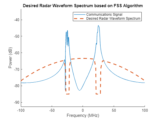
Figure contains an axes object. The axes object with title Desired Radar Waveform Spectrum based on FSS Algorithm, xlabel Frequency (MHz), ylabel Power (dB) contains 2 objects of type line. These objects represent Communications Signal, Desired Radar Waveform Spectrum.

This plot illustrates that using this FSS algorithm, a desired radar waveform spectrum is generated that has notches in the region of highest communications signal power. A radar waveform with this spectrum would substantially reduce mutual interference between the radar and communications systems.

Notched Waveform Design and Analysis

After the desired spectrum is determined based on the FSS algorithm, a waveform must be generated that conforms to this spectrum. In this example, we use a PRO-FM waveform [1]. This is a noise waveform that contains desirable range sidelobe characteristics and is amenable to spectral notching due to the nature of its construction. These characteristics make this a versatile waveform that is a good candidate for spectrum sharing. To generate this waveform, a seed waveform is optimized iteratively to contain a desired frequency spectrum shape and uniform amplitude [3].

Generate Initial PCFM Waveform

In the process of generating a PRO-FM waveform, you start with a seed waveform made up of data symbols with random phase. The frequency spectrum of this waveform is dictated by the symbol rate. This seed waveform is a Polyphase-Coded FM (PCFM) waveform that has random frequency values within the desired frequency band throughout the duration of the pulse [4]. This type of waveform has been shown to be amenable to spectral shaping via the PRO-FM process [3].

The transmit waveform has a design bandwidth of 100 MHz, a pulse width of 2 us, a pulse repetition interval of 80 us, and a coherent processing interval (CPI) with 200 pulses.

rng("default")            % Set random number generator for reproducibility 
bandwidth = 100e6;        % Design bandwidth is 100 MHz
pulseWidth = 2e-6;        % Pulse width is 2 us
pri = 80e-6;              % PRI is 80 us
numPulses = 200;          % 200 pulses in a CPI

% Sample at 2x our design bandwidth
sampleRate = 2*bandwidth;

The following steps describe the process of generating the PCFM waveform with random frequencies throughout the pulse duration.

Randomly generate N+1 symbol phases $θ, where θ \in [- π π]$
Calculate N phases differences $α_{n}, where α_{n} = θ_{n} - θ_{n - 1}$ for n = 1,...,N. If $| α_{n} |$ > $π$ , $α_{n} = α_{n} - 2 π * sgn (α_{n})$ . In this equation, $sgn$ is the sign function.
Create an impulse train of phase differences using the equation $\sum_{n = 1}^{N} α_{n} * δ (t - (n - 1) T_{p})$ , where $T_{p}$ is the time separation between impulses and $δ (t)$ is a unit impulse at time t. This impulse train carries the random frequency information of the desired signal.
Filter the impulse train to create smooth frequency transitions between samples. In this case, we use a raised-cosine filter.
Integrate the filtered impulse train F(t) from 0 to t to recover the desired signal phase values. Assume $θ_{0}$ as the initial condition: $P (t) = \int_{0}^{t} F (t) d τ +$ $θ_{0}$
Recover the complex signal from the phase values: $s (t) = e^{iP (t)}$ , where s(t) is the final PCFM waveform.

The following code generates the seed waveform using the algorithm described above, and plots the waveform characteristics.

% Generate the PCFM seed waveform
pcfmWaveform = helperSeedWaveform(bandwidth,pulseWidth,sampleRate,numPulses);

% Plot the waveform spectrogram for a single pulse
stft(pcfmWaveform(:,1),sampleRate); title('PCFM Seed Waveform Spectrogram');

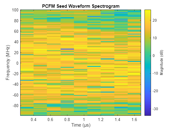
Figure contains an axes object. The axes object with title PCFM Seed Waveform Spectrogram, xlabel Time (μs), ylabel Frequency (MHz) contains an object of type image.

The spectrogram of the PCFM signal shows that the frequency is randomly distributed as a function of time.

% Plot the seed waveform power spectrum averaged across pulses
pSeed = pspectrum(pcfmWaveform,sampleRate);
pSeedMean = mean(pSeed,2);
fSeed = helperSpectrumFrequencies(sampleRate,numel(pSeedMean));
plot(fSeed/10^6,pow2db(pSeedMean)); xlabel('Frequency (MHz)'); ylabel('Power Spectrum (dB)'); title('PCFM Seed Waveform Mean Spectrum Power');

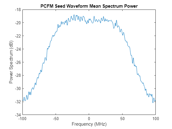
Figure contains an axes object. The axes object with title PCFM Seed Waveform Mean Spectrum Power, xlabel Frequency (MHz), ylabel Power Spectrum (dB) contains an object of type line.

The power spectrum clearly illustrates that more power is concentrated towards the center of the spectrum, although the spectral shape is not Gaussian.

% Plot the ambiguity function for a single pulse
ambgfun(pcfmWaveform(:,1),sampleRate,1/pulseWidth); title('PCFM Seed Waveform Ambiguity Function'); ylim([-3 3]); xlim([-0.3 0.3]);

Figure contains an axes object. The axes object with title PCFM Seed Waveform Ambiguity Function, xlabel Delay tau blank (us), ylabel Doppler f indexOf d baseline blank (MHz) contains an object of type contour.

Some Range-Doppler sidelobes are visible in the ambiguity function and appear to be distributed randomly, which is not unexpected due to the nature of the waveform's construction.

Generate Notched Waveform

The generation of the notched waveform is achieved using the shapespectrum function. The desired spectrum is the notched spectrum that was generated using the FSS algorithm and the initial waveform is set to the PCFM waveform that was created in the previous section [1].

% Generate a notched frequency spectrum
proFmNotched = zeros(numSamples,numPulses);
notchedSpectrum = pow2db(desiredRadarSpectrum);
for iPulse = 1:numPulses
    initialWaveform = pcfmWaveform(:,iPulse);
    proFmNotched(:,iPulse) = shapespectrum(notchedSpectrum,initialWaveform,DesiredSpectrumRange='centered');
end

% Plot the waveform spectrogram for a single pulse
stft(proFmNotched(:,1),sampleRate); title('PRO-FM Notched Waveform Spectrogram');

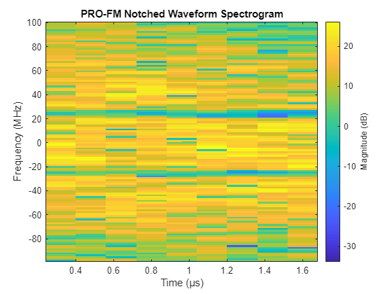
Figure contains an axes object. The axes object with title PRO-FM Notched Waveform Spectrogram, xlabel Time (μs), ylabel Frequency (MHz) contains an object of type image.

The PRO-FM spectrogram still shows a randomly varying frequency throughout the duration of the pulse, although the power is more concentrated towards the center of the distribution and there are regions of low power where the frequency spectrum notches are.

% Plot the PRO-FM waveform power spectrum averaged across pulses
pProFm = pspectrum(proFmNotched,sampleRate);
pProFmMean = mean(pProFm,2);
fProFm = helperSpectrumFrequencies(sampleRate,numel(pProFmMean));
plot(fProFm/10^6,pow2db(pProFmMean)); xlabel('Frequency (MHz)'); ylabel('Power Spectrum (dB)'); title('PRO-FM Notched Waveform Mean Spectrum Power');

Figure contains an axes object. The axes object with title PRO-FM Notched Waveform Mean Spectrum Power, xlabel Frequency (MHz), ylabel Power Spectrum (dB) contains an object of type line.

The power spectrum clearly illustrates the Gaussian shape of the spectrum and the presence of notches at the locations determined by FSS.

% Plot the ambiguity function for a single pulse
ambgfun(proFmNotched(:,1),sampleRate,1/pulseWidth); title('PRO-FM Notched Waveform Ambiguity Function'); ylim([-3 3]); xlim([-0.3 0.3]);

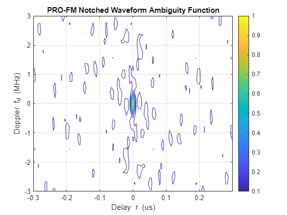
Figure contains an axes object. The axes object with title PRO-FM Notched Waveform Ambiguity Function, xlabel Delay tau blank (us), ylabel Doppler f indexOf d baseline blank (MHz) contains an object of type contour.

The ambiguity function shows the presence of significant Range-Doppler sidelobes. The issue of sidelobes in the waveform ambiguity function is largely mitigated by altering the transmit waveform in a CPI on a pulse-to-pulse basis. Using this variable waveform approach, the location of these Range-Doppler sidelobes change throughout a CPI and their impact on performance is significantly reduced [1].

Impact of Notches on Radar Performance

The previous two sections in this example showed how to determine the waveform transmission region using an FSS algorithm and how to subsequently generate a PRO-FM notched waveform using the desired transmission spectrum obtained from the FSS algorithm.

This section will analyze the impact that waveform notching has on radar performance by simulating the transmission of the notched vs. unnotched waveforms in the presence of the communications signal.

The communications signal is assumed to occupy a fixed region for the duration of a radar CPI for simplicity. This example could be adjusted so that the location of the OFDM transmission changes throughout the CPI, but for this example only the simplest case is examined. The communications signal generated in the prior section is reused here.

Generate Unnotched and Notched Waveforms

In order to analyze the impact of waveform notching on radar performance, we generate unnotched and notched PRO-FM waveforms. A new waveform is generated for each pulse in the CPI. The notched waveform has notches placed at the frequencies determined using the FSS algorithm.

% Generate notched and unnotched waveforms for a 200 pulse CPI.
unnotchedWaveformCpi = helperGenerateUnnotchedWaveform(bandwidth,pulseWidth,sampleRate,numPulses);
notchedWaveformCpi = helperGenerateNotchedWaveform(bandwidth,pulseWidth,sampleRate,numPulses,notchFrequencies);

Plot the unnotched and notched waveform spectrums alongside the communications signal spectrum to visualize the spectrum of the waveforms that are being used for transmission in this section.

% Plot communications signal as well as notched and unnotched waveform
helperPlotCommsWithRadar(commsSignal,unnotchedWaveformCpi,notchedWaveformCpi,peakSinrDb,sampleRate);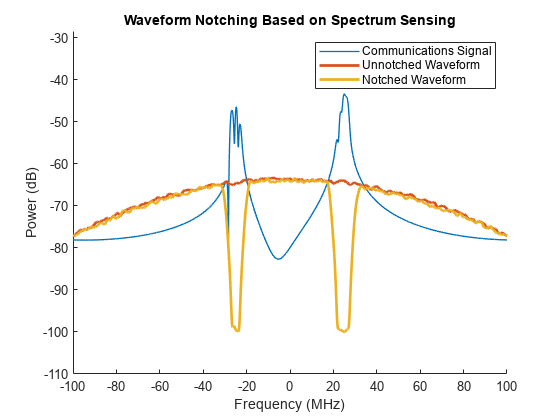

Figure contains an axes object. The axes object with title Waveform Notching Based on Spectrum Sensing, xlabel Frequency (MHz), ylabel Power (dB) contains 3 objects of type line. These objects represent Communications Signal, Unnotched Waveform, Notched Waveform.

Simulate Transmission of Waveforms and Analyze Performance

In this section, we run a simulation to analyze the performance of the unnotched and notched waveforms in the absence and presence of the communications signal.

Prior to running this simulation, we create a set of transmit radar waveforms combined with communications waveforms. An alternative approach would be to add the communications signal to the entire receive pulse instead of just the transmit waveform. In this case, the communications signal is added only to the transmit waveform for simplicity to easily maintain the desired SINR on receive. Prior to combining the radar waveform with the communications waveform, this function scales the signals so that the SINR is set to the desired level.

% Add communications signal to waveforms with desired SINR
notchedWaveformCpiWithComms = helperCombineSignals(notchedWaveformCpi,commsSignal,peakSinrDb);
unnotchedWaveformCpiWithComms = helperCombineSignals(unnotchedWaveformCpi,commsSignal,peakSinrDb);

Once the radar waveforms have been generated and combined with the interfering communications waveform, set up target locations and velocities. Use 6 targets total with some moving towards the platform and some moving away from the platform.

% Set up target ranges and velocities
targetPositions = [[500;0;0],[500;0;0],[600;0;0],...
                   [600;0;0],[700;0;0],[700;0;0]];

targetVelocities = [[5;0;0],[-5;0;0],[10;0;0],...
                    [-10;0;0],[15;0;0],[-15;0;0]];

% Velocity and range limits for the Range-Doppler Plot
rLim = [450 750];
vLim = [-30 30];

After generating the waveforms and setting up the target properties, run the simulation of a single CPI and plot the Range-Doppler response of the unnotched and notched waveforms in the absence and presence of interference. For more information on simulating the transmission of custom waveforms, see Waveform Design to Improve Range Performance of an Existing System.

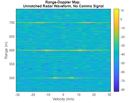
The first two plots show the Range-Doppler map for the notched and unnotched waveforms in the absence of the communications signal.

% Run simulation and plot Range-Doppler response for unnotched waveform
% without communications signal
[rdUnnotchedNoComms,rdRange,rdVelocity] = helperRunSimulation(unnotchedWaveformCpi,unnotchedWaveformCpi,fc,sampleRate,pri,targetPositions,targetVelocities,"Unnotched Radar Waveform, No Comms Signal",vLim,rLim);

Figure contains an axes object. The axes object with title Range-Doppler Map: Unnotched Radar Waveform, No Comms Signal, xlabel Velocity (m/s), ylabel Range (m) contains an object of type image.

% Run simulation and plot Range-Doppler response for notched waveform
% without communications signal
rdNotchedNoComms = helperRunSimulation(notchedWaveformCpi,notchedWaveformCpi,fc,sampleRate,pri,targetPositions,targetVelocities,"Notched Radar Waveform, No Comms Signal",vLim,rLim);

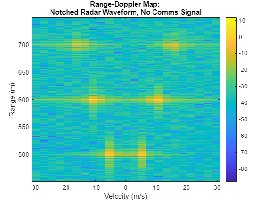
Figure contains an axes object. The axes object with title Range-Doppler Map: Notched Radar Waveform, No Comms Signal, xlabel Velocity (m/s), ylabel Range (m) contains an object of type image.

Higher range sidelobes are evident in the notched waveform when compared with the unnotched waveform. Without the presence of the communications signal, the performance of the unnotched waveform qualitatively appears to be better than the notched waveform, which is expected.

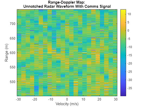
The plots below show performance of the notched and unnotched waveforms in the presence of the communications signal. This is where the performance benefits of the notched waveform are evident.

% Run simulation and plot Range-Doppler response for unnotched waveform
% with communications signal
rdUnnotchedWithComms = helperRunSimulation(unnotchedWaveformCpiWithComms,unnotchedWaveformCpi,fc,sampleRate,pri,targetPositions,targetVelocities,"Unnotched Radar Waveform With Comms Signal",vLim,rLim);

Figure contains an axes object. The axes object with title Range-Doppler Map: Unnotched Radar Waveform With Comms Signal, xlabel Velocity (m/s), ylabel Range (m) contains an object of type image.

% Run simulation and plot Range-Doppler response for unnotched waveform
% with communications signal
rdNotchedWithComms = helperRunSimulation(notchedWaveformCpiWithComms,notchedWaveformCpi,fc,sampleRate,pri,targetPositions,targetVelocities,"Notched Radar Waveform With Comms Signal",vLim,rLim);

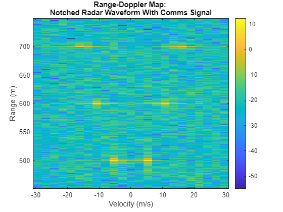
Figure contains an axes object. The axes object with title Range-Doppler Map: Notched Radar Waveform With Comms Signal, xlabel Velocity (m/s), ylabel Range (m) contains an object of type image.

When using an unnotched waveform in the presence of the communications signal, the targets become difficult to distinguish on the Range-Doppler map. Contrast this with the notched waveform Range-Doppler map, where the targets are still clearly visible.

In order to quantify the performance difference between each test case, the average SINR of all the targets is compared. For this example, the noise level is calculated in an unoccupied region from 620 to 680 meters in range and -10 to 10 m/s in Doppler velocity.

% Use 620 to 680 m, -10 to 10 m/s Doppler, as the region to calculate noise
% power (excluding target locations)
noiseRange = [620 680];
noiseVelocity = [-10 10];

% Display a table of target SINR values as well as differences between each
% test case and the base case of unnotched waveform no communications signal.
T = helperGetSinrTable(rdUnnotchedNoComms,rdNotchedNoComms,rdUnnotchedWithComms,rdNotchedWithComms,rdRange,rdVelocity,targetPositions,targetVelocities,noiseRange,noiseVelocity);
disp(T);

                                    SINR at Target Locations (dB)    Delta with Unnotched, No Comms Signal
                                    _____________________________    _____________________________________

    Unnotched, No Comms Signal                 45.797                                     0               
    Notched, No Comms Signal                   43.724                               -2.0725               
    Unnotched, With Comms Signal               15.623                               -30.173               
    Notched, With Comms Signal                 28.519                               -17.278

This quantitative analysis confirms what is observed qualitatively in the Range-Doppler plots - without any communications signal, the unnotched radar waveform has a marginally higher SINR than the notched radar waveform. However, when the communications signal is present, the SINR of the notched radar waveform is significantly higher than that of the unnotched radar waveform.

Using this type of notching, radar systems can coexist with communication systems while continuing to detect targets effectively.

Summary

In this example, you learned how to implement a fast spectrum sensing algorithm to determine the desirable frequency transmission region, as well a waveform notching algorithm to limit transmit frequency to the desirable region. The effectiveness of this approach was then analyzed by simulating the transmission, propagation, and reception of the custom waveform in the presence of a communications signal. This type of workflow may become more common as the need for coexistence schemes between radar and communications systems become more pressing in the future.

References

[1] Ravenscroft et al. Experimental demonstration and analysis of cognitive spectrum sensing and notching for radar. IET Radar, Sonar & Navigation. 2018.

[2] Martone et al. Spectrum Allocation for Non-Cooperative Radar Coexistence. IEEE Transactions on Aerospace and Electronic Systems. 2018.

[3] Jakabosky et al. Waveform Design and Receive Processing for Nonrecurrent Nonlinear FMCW Radar. IEEE. 2015.

[4] Blunt et al. Polyphase-Coded FM (PCFM) Radar Waveforms, Part 1: Implementation. IEEE. 2014.

Helper Functions

The following group of helper functions implement the spectrum sensing algorithms discussed in [2].

function mesoBands = helperMesoBands(interferenceSpectrumPower,powerThresholdDb,minBandwidth,sampleRate)
    % Get the initial meso bands in high and low power
    initialMesoBands = helperInitialMesoBands(interferenceSpectrumPower,powerThresholdDb);

    % Merge high and low power meso bands
    mesoBands = helperMergeMesoBands(initialMesoBands,minBandwidth,sampleRate);
end

function initialMesoBands = helperInitialMesoBands(spectrumPower,powerThresholdDb)
    % Generate initial meso-bands from a power spectrum for a given
    % threshold    
    
    % Get the spectrum power in dB
    spectrumPowerDb = pow2db(spectrumPower);
        
    % Hold meso-band start/end index, and whether it is high power
    initialMesoBands = [];
    
    % Initialize loop parameters
    spectrumSamples = length(spectrumPowerDb);
    iStart = 1;
    mesoBandIdx = 1;
    
    for iSample = 1:spectrumSamples
        % Check if the current band start and stop powers are high
        startHighPower = spectrumPowerDb(iStart) > powerThresholdDb;
        stopHighPower = spectrumPowerDb(iSample) > powerThresholdDb;
    
        % If the start and stop values are in the same power band, advance the
        % stop index continue, otherwise this is the end of a meso-band.
        if startHighPower ~= stopHighPower
            initialMesoBands = helperSetMesoBands(initialMesoBands,mesoBandIdx,iStart,iSample-1,startHighPower);
            mesoBandIdx = mesoBandIdx + 1;
            iStart = iSample;
        end
    end
    
    % Set the last meso-band
    initialMesoBands = helperSetMesoBands(initialMesoBands,mesoBandIdx,iStart,spectrumSamples,spectrumPowerDb(iStart) > powerThresholdDb);

end

function mergedMesoBands = helperMergeMesoBands(initialMesoBands,minBandwidth,sampleRate)
    % Merge low power meso-bands for a given minimum bandwidth
    
    % Get the number of samples in the spectrum
    interferenceSamples = initialMesoBands(end).iStop-initialMesoBands(1).iStart+1;
    
    % Calculate the minimum number of samples based on minimum bandwidth
    Lmin = floor(interferenceSamples/sampleRate*minBandwidth);
    
    % Set the initial index based on whether 1st meso-band is high power
    mergedMesoBands = initialMesoBands;
    if mergedMesoBands(1).HighPower
        currentIdx = 2;
    else
        currentIdx = 1;
    end
    
    [~,numBands] = size(mergedMesoBands);
    
    % Merge low power bands if they are too narrow
    while currentIdx <= numBands
        currentBand = mergedMesoBands(currentIdx);
        currentBandSampleNum = currentBand.iStop - currentBand.iStart + 1;
        if currentBandSampleNum < Lmin
            [mergedMesoBands,currentIdx,numBands] = mergeSingleMesoBand(mergedMesoBands,currentIdx);
        else
            % Increment by 2 to ensure we only look at low power bands
            currentIdx = currentIdx + 2;
        end
    end

    % Merge the meso-band at the given index with neighbors
    function [newMesoBands,currentIdx,newNumBands] = mergeSingleMesoBand(mesoBands,currentIdx)
        [~,initialNumBands] = size(mesoBands);
        
        % Determine the range of bands to combine. This is different if we
        % are on the first or the last meso-band.
        if currentIdx == 1
            newNumBands = initialNumBands-1;
            currentIdx = 2;
            combineBandRange = 1:2;
        elseif currentIdx == initialNumBands
            newNumBands = initialNumBands-1;
            combineBandRange = initialNumBands-1:initialNumBands;
        else
            newNumBands = initialNumBands-2;
            combineBandRange = currentIdx-1:currentIdx+1;
        end
        
        % Get the start and end index of the meso-bands that are being
        % combined.
        startIdx = mesoBands(combineBandRange(1)).iStart;
        endIdx = mesoBands(combineBandRange(end)).iStop;
        
        % Create the new meso-band, which is always high power
        newBand = helperCreateMesoBand(startIdx,endIdx,true);
    
        % Get the indexes of the prior and next bands after combining
        priorBandIdx = combineBandRange(1)-1;
        nextBandIdx = combineBandRange(end)+1;
    
        % Set the new meso-bands after combining the specified band
        newMesoBands = [];
        if priorBandIdx > 0
            newMesoBands = mesoBands(1:priorBandIdx);
        end
    
        newMesoBands = [newMesoBands,newBand];
    
        if nextBandIdx <= initialNumBands
            newMesoBands = [newMesoBands,mesoBands(nextBandIdx:end)];
        end  
    end
end

function mesoBands = helperSetMesoBands(mesoBands,mesoBandIdx,iStart,iStop,highPower)
    % Create meso-band struct row, add it to the meso-bands struct
    
    if isempty(mesoBands)
        mesoBands = helperCreateMesoBand(iStart,iStop,highPower);
    else
        mesoBands(mesoBandIdx) = helperCreateMesoBand(iStart,iStop,highPower);
    end
end

function newBand = helperCreateMesoBand(startIdx,endIdx,highPower)
    % Create a new meso-band

    newBand = struct('iStart',startIdx,'iStop',endIdx,'HighPower',highPower);
end

function a = helperPlotMesoBands(spectrumPower,mesoBands,threshold,spectrumFrequencies,plotTitle,plotXlim)
    % Plot meso-bands along with the frequency spectrum
    
    % Offset the high and low power bands by 10 dB for display purposes
    offset = 10;
    
    % Get the spectrum power in dB
    spectrumPowerDb = pow2db(spectrumPower);
    
    % Get the start and stop idxs
    threshIdxs = [mesoBands(1).iStart mesoBands(end).iStop];
    
    % Get spectrum frequencies in MHz
    spectrumFrequencies = spectrumFrequencies/1e6;
    
    % Plot the spectrum and meso-bands
    a = axes(figure);
    hold(a,"on");
    lThresh = plot(a,spectrumFrequencies(threshIdxs),[threshold threshold],'DisplayName','Threshold','LineStyle','--','Color','k','LineWidth',1);
    lSpec = plot(a,spectrumFrequencies,spectrumPowerDb,'DisplayName','Measured Spectrum','LineWidth',1,'Color','b');
    hold(a,"off");
    lLow = plotMesoBandLevel(mesoBands(~[mesoBands.HighPower]),threshold,threshold-offset,spectrumFrequencies,"Low Power Meso-Band","g",a);
    lHigh = plotMesoBandLevel(mesoBands([mesoBands.HighPower]),threshold,threshold+offset,spectrumFrequencies,"High Power Meso-Band","r",a);
    ylabel(a,'Power (dB)')
    xlabel(a, 'Frequency (MHz)')
    legend(a,[lSpec,lLow,lHigh,lThresh],"Location","southeast");
    title(a,plotTitle);
    xlim(a,plotXlim);
    
    % Plot high or low power meso-bands
    function l = plotMesoBandLevel(mesoBands,threshold,plotPower,freq,description,color,a)
        [~,numBands] = size(mesoBands);
    
        hold(a,"on");
        for iBand = 1:numBands
            start = mesoBands(iBand).iStart;
            stop = mesoBands(iBand).iStop;
            range = start:stop;
            x = [start,range,stop];
            y = [threshold,repmat(plotPower,[1,length(range)]),threshold];
            l = plot(a,freq(x),y,'DisplayName',description,'Color',color,'LineWidth',2);
        end
        hold(a,"off");
    end
end

function notchFrequencies = helperTxNotchFrequencies(mesoBands,signalSpectrumPower,interferenceSpectrumPower,tau,alpha,sampleRate)
    % Determine notch frequency locations by maximizing the objective function
    % for all combinations of messo-bands
    % Determine the frequencies to notch
                
    % Calculate the tx band objective values
    txBandObjValues = getTxBandObjectiveValues(mesoBands,signalSpectrumPower,interferenceSpectrumPower,tau,sampleRate);
    
    % Calculate normalized objective values for each tx band
    txBandObjValuesNorm = normalizeTxBandObjectiveValues(txBandObjValues);
    
    % Get the transmit region with the max objective function
    txMesoBands = getMaxObjectiveBands(txBandObjValuesNorm,alpha);
    
    % Get the notch frequency regions
    spectrumFrequencies = helperSpectrumFrequencies(sampleRate,numel(interferenceSpectrumPower));
    notchFrequencies = getNotchFrequencyFromTxRegion(mesoBands,txMesoBands,spectrumFrequencies);
    
    function txBandObjectives = getTxBandObjectiveValues(mesoBands,signalSpectrumPower,interferenceSpectrumPower,tau,sampleRate)
        % Get all possible band combinations
        [~,numBands] = size(mesoBands);
        possibleTxBands = getAllPossibleTxBands(numBands);
    
        % Calculate objectives for each tx band combination
        txBandObjectives = calculateTxBandObjectiveValues(possibleTxBands,mesoBands,signalSpectrumPower,interferenceSpectrumPower,tau,sampleRate);
    
        function possibleBands = getAllPossibleTxBands(numBands)
            % Get every permutation of meso-band combinations
            possibleBands = struct('BandCombo',[],'SINR',[],'Bandwidth',[]);
            bandComboIdx = 1;
            
            availableBands = 1:numBands;
            
            for iBandCombos = 1:numBands
                combos = nchoosek(availableBands,iBandCombos);
                [numCombos,~] = size(combos);
                for iCombo = 1:numCombos
                    possibleBands(bandComboIdx,1).BandCombo = combos(iCombo,:);
                    bandComboIdx = bandComboIdx+1;
                end
            end
        end
    
        function txBandCalculations = calculateTxBandObjectiveValues(txBandCalculations,mesoBands,signalSpectrumPower,interferenceSpectrumPower,tau,sampleRate)
            % Calculate the objective functions for each possible meso-band combination
            
            [numPossibleBands,~] = size(txBandCalculations);
    
            % Get the frequency values for interference and signal spectrums
            fInterference = helperSpectrumFrequencies(sampleRate,numel(interferenceSpectrumPower));
            fStepInterference = fInterference(2)-fInterference(1);
            fSignal = helperSpectrumFrequencies(sampleRate,numel(signalSpectrumPower));
            fStepSignal = fSignal(2)-fSignal(1);
            
            % Set the sinr and bandwidth for all possible bands
            for iBandCombo = 1:numPossibleBands
                % Get the indexes of the interference and signal in this
                % meso-band
                bands = txBandCalculations(iBandCombo).BandCombo;
                [intBandIdxs,sigBandIdxs] = getBandIdxs(mesoBands,bands,fInterference,fSignal);
        
                % Get the power contained in the signal. Multiplication by tau in order to
                % capture effect of pulse width.
                mesoBandSignalPower = sum(signalSpectrumPower(sigBandIdxs))*tau*fStepSignal;
                
                % Get the power contained in the interference
                mesoBandInterferencePower = sum(interferenceSpectrumPower(intBandIdxs))*fStepInterference;
                
                % Calculate SINR and bandwidth for this mesoband
                sinr = mesoBandSignalPower / mesoBandInterferencePower;
                bandwidth = length(intBandIdxs)*fStepInterference;
        
                % Store the SINR and bandwidth
                txBandCalculations(iBandCombo).SINR = sinr;
                txBandCalculations(iBandCombo).Bandwidth = bandwidth;
            end
    
            function [intBandIdxs,sigBandIdxs] = getBandIdxs(mesoBands,bands,fInterference,fSignal)
            % Get band indexes from meso-bands.
                intBandIdxs = [];
                sigBandIdxs = [];
                for iBand = 1:length(bands)
                    currentIntIdxs = mesoBands(bands(iBand)).iStart:mesoBands(bands(iBand)).iStop;
                    currentSigIdxs = getIdxFromFreq(fInterference(currentIntIdxs(1)),fInterference(currentIntIdxs(end)),fSignal);
                    intBandIdxs = [intBandIdxs,currentIntIdxs];
                    sigBandIdxs = [sigBandIdxs,currentSigIdxs];
                end
    
                function idxs = getIdxFromFreq(startFreq,stopFreq,freqSamples)
                % Get the frequency sample indexes from start and stop frequencies
                    startIdxs = find(startFreq <= freqSamples);
                    stopIdxs = find(stopFreq >= freqSamples);
                    idxs = (startIdxs(1):stopIdxs(end));
                end
            end
        end
    end
    
    function txBandsNormValues = normalizeTxBandObjectiveValues(txBandsObjValues)
        % Normalize tx band objective values
        normColumns = {'SINR','Bandwidth'};
        txBandsNormValues = normalizeColumns(txBandsObjValues,normColumns);
            
        function txBandsNorm = normalizeColumns(txBands,normColumnNames)
            txBandsNorm = txBands;    
            [rows,~] = size(txBands);
            
            for iColumn = 1:length(normColumnNames)
                name = normColumnNames{iColumn};
                normName = ['norm',name];
                maxValue = max([txBands.(name)]);
                for iRow = 1:rows
                    txBandsNorm(iRow).(normName) = txBands(iRow).(name)/maxValue;
                end
            end
        end
    end
    
    function txBands = getMaxObjectiveBands(normObjective,alpha)
        % Get the idxs that maximize the objective function
        maxObjective = -Inf;
        maxObjectiveRow = 0;
        [rows,~] = size(normObjective);
    
        for iRow = 1:rows
            objective = alpha*normObjective(iRow).normSINR + (1-alpha)*normObjective(iRow).normBandwidth;
            if objective > maxObjective
                maxObjectiveRow = iRow;
                maxObjective = objective;
            end
        end
    
        txBands = normObjective(maxObjectiveRow).BandCombo;
    end
    
    function notchFrequency = getNotchFrequencyFromTxRegion(mesoBands,txMesoBands,spectrumFrequencies)
        % Get the frequency ranges of the notches based on the selected tx
        % meso-bands
        notchMesoBands = mesoBands;
        notchMesoBands(txMesoBands) = [];
    
        [~,numNotches] = size(notchMesoBands);
        notchFrequency = zeros(numNotches,2);
        for iNotch = 1:numNotches
            bandStart = notchMesoBands(iNotch).iStart;
            bandStop = notchMesoBands(iNotch).iStop;
            notchFrequency(iNotch,:) = [spectrumFrequencies(bandStart) spectrumFrequencies(bandStop)];
        end
    end
end

The following group of helper functions implement the waveform generation algorithms.

function waveform = helperGenerateUnnotchedWaveform(bandwidth,pulseWidth,sampleRate,numPulses)
    % Generate an unnotched waveform using the approach described in [1].
    
    % Call helperGenerateNotchedWaveform with empty notch frequencies
    notchFrequencies = [];
    waveform = helperGenerateNotchedWaveform(bandwidth,pulseWidth,sampleRate,numPulses,notchFrequencies);
end

function waveform = helperGenerateNotchedWaveform(bandwidth,pulseWidth,sampleRate,numPulses,notchFrequencies)
    % Generate a notched waveform using the approach described in [1].
    
    % Generate the seed waveform
    pcfmWaveform = helperSeedWaveform(bandwidth,pulseWidth,sampleRate,numPulses);
    
    % Calculate the number of samples in the pulse, and get the frequencies in
    % the spectrum
    numSamples = pulseWidth*sampleRate;
    
    % Generate the unnotched Gaussian spectrum.
    unnotchedSpectrum = gausswin(numSamples);
    
    % Notch the spectrum
    notchedSpectrum = helperNotchSpectrum(unnotchedSpectrum,sampleRate,notchFrequencies);
    
    % Generate the notched waveform
    waveform = zeros(size(pcfmWaveform));
    for iPulse = 1:numPulses
        waveform(:,iPulse) = shapespectrum(pow2db(notchedSpectrum),pcfmWaveform(:,iPulse),DesiredSpectrumRange="centered");
    end
end

function pcfmWaveform = helperSeedWaveform(bandwidth,pulseWidth,sampleRate,numPulses)
    % Generate a PCFM waveform with randomized frequencies following the
    % process described in [4].
    
    % Get the number of samples in a symbol and the number of symbols in a
    % pulse
    samplesPerPulse = pulseWidth*sampleRate;
    samplesPerSymbol = sampleRate/bandwidth;
    symbolsPerPulse = samplesPerPulse/samplesPerSymbol;
    samplesPerPulse = samplesPerSymbol*symbolsPerPulse;
    
    % Perform randomized PCFM steps
    randomPhases = 2*pi*(rand(symbolsPerPulse+1,numPulses)-0.5);
    
    % Calculate the phase difference
    phaseDifference = pcfmCalculatePhaseDifference(randomPhases);
    
    % Generate impulse train
    impulseTrain = pcfmGenerateImpulseTrain(phaseDifference,numPulses,samplesPerSymbol,samplesPerPulse);
    
    % Filter impulses
    filteredImpulseTrain = pcfmFilterImpulseTrain(impulseTrain,samplesPerSymbol);
    
    % Integrate to get phase
    pcfmPhases = randomPhases(1,:) + cumtrapz(filteredImpulseTrain,1);
    
    % Generate samples based on phase
    pcfmWaveform = exp(1i*pcfmPhases);
    
    % Get the phase difference of the random phases
    function phaseDifference = pcfmCalculatePhaseDifference(randomPhases)
        phaseDifference = diff(randomPhases,[],1);
        greaterThanPi = abs(phaseDifference) > pi;
        phaseDifference(greaterThanPi) = phaseDifference(greaterThanPi) - 2*pi*sign(phaseDifference(greaterThanPi));
    end
    
    % Get the impulse train representing frequency
    function impulseTrain = pcfmGenerateImpulseTrain(phaseDifference,numPulses,samplesPerSymbol,totalSamples)
        impulseTrain = zeros(totalSamples,numPulses);
        impulseTrain(1:samplesPerSymbol:totalSamples,:) = phaseDifference;
    end
    
    % Get the filtered impulse train representing frequency
    function filteredImpulseTrain = pcfmFilterImpulseTrain(impulseTrain,samplesPerSymbol)
        raisedCosFilter = rcosdesign(0.25,6,samplesPerSymbol)';
    
        [rows,cols] = size(impulseTrain);
        filteredImpulseTrain = zeros(rows,cols);
        for iCol = 1:cols
            filteredImpulseTrain(:,iCol) = conv(impulseTrain(:,iCol),raisedCosFilter,'same');
        end
    end
end

function notchedSpectrum = helperNotchSpectrum(initialSpectrum,sampleRate,notchFrequencies)
    % Insert notches into the given spectrum. Use Tukey Tapers following the
    % process described in [4].
    
    % Get the spectrum in dB.
    logSpectrum = pow2db(initialSpectrum);
    
    % Get the spectrum frequency samples
    spectrumFrequencies = helperSpectrumFrequencies(sampleRate,numel(initialSpectrum));
    
    % Set the notch floor to -85 dB
    minValue = -85;
    
    % Get the number of samples in the spectrum
    numSamples = length(initialSpectrum);
    
    % taper is B/32, number if samples is 2B, so taper is samples/64
    taperLength = ceil(numSamples/64);
    
    % Get the indexes of the notch frequencies in the spectrum
    notchIdxs = getNotchStartEndIdx(notchFrequencies,spectrumFrequencies);
    [notchNum,~] = size(notchIdxs);
    
    % For each notch, update the spectrum
    for iNotch = 1:notchNum
        idxs = notchIdxs(iNotch,:);
        logSpectrum(idxs(1):idxs(end)) = minValue;
        
        % set tukey taper on leading and trailing edges of notch
        fallingTaperStart = idxs(1)-taperLength;
        fallingTaperStartValue = logSpectrum(fallingTaperStart);
        fallingTaper = createTukeyTaper(taperLength,fallingTaperStartValue,minValue);
        logSpectrum(fallingTaperStart:idxs(1)) = fallingTaper;
    
        risingTaperEnd = idxs(end)+taperLength;
        risingTaperEndValue = logSpectrum(risingTaperEnd);
        risingTaper = createTukeyTaper(taperLength,minValue,risingTaperEndValue);
        logSpectrum(idxs(end):risingTaperEnd) = risingTaper;
    end
    
    % Return spectrum power as amplitude
    notchedSpectrum = db2pow(logSpectrum);
    
    function taper = createTukeyTaper(numSamples,startValue,endValue)
    % Insert a taper where spectral notches occur.
        height = abs(startValue-endValue)/4;
        lowestValue = max([startValue,endValue])-height;
        if startValue > endValue
            flipTaper = false;
        else
            flipTaper = true;
        end
    
        % create taper
        taper = cos(0.5*pi/numSamples*(0:numSamples));
        
        % stretch taper to height
        taper = taper*height;
    
        % move taper down to end value
        taper = taper+lowestValue;
    
        if flipTaper
            taper = flip(taper);
        end
    end
    
    % Get the start and end index of the notch frequencies
    function notchIdxs = getNotchStartEndIdx(notchFreq,spectrumFrequencies)
        [numNotches,~] = size(notchFreq);
        notchIdxs = zeros(numNotches,2);
    
        for iNotchFreq = 1:numNotches
            notchStart = notchFreq(iNotchFreq,1);
            notchEnd = notchFreq(iNotchFreq,2);
    
            aboveNotchStart = find(spectrumFrequencies >= notchStart);
            belowNotchEnd = find(spectrumFrequencies <= notchEnd);
            notchIdxs(iNotchFreq,:) = [aboveNotchStart(1) belowNotchEnd(end)];
        end
    end
end