Transmitter

Transmitter Object

The phased.Transmitter object lets you model key components of the radar equation including the peak transmit power, the transmit gain, and a system loss factor.

While the preceding functionality is important in applications dependent on amplitude such as signal detectability, Doppler processing depends on the phase of the complex envelope. In order to accurately estimate the radial velocity of moving targets, it is important that the radar operates in either a fully coherent or pseudo-coherent mode. In the fully coherent, or coherent on transmit, mode, the phase of the transmitted pulses is constant. Constant phase provides you with a reference to detect Doppler shifts.

A transmitter that applies a random phase to each pulse creates phase noise that can obscure Doppler shifts. If the components of the radar do not enable you to maintain constant phase, you can create a pseudo-coherent, or coherent on receive radar by keeping a record of the random phase errors introduced by the transmitter. The receiver can correct for these errors by modulation of the complex envelope. The phased.Transmitter object enables you to model both coherent on transmit and coherent on receive behavior.

The transmitter object has the following modifiable properties:

PeakPower — Peak transmit power in watts
Gain — Transmit gain in decibels
LossFactor — Loss factor in decibels
InUseOutputPort — Track transmitter's status. Setting this property to true outputs a vector of 1s and 0s indicating when transmitter is on and off. In a monostatic radar, the transmitter and receiver cannot operate simultaneously.
CoherentOnTransmit — Preserve coherence among transmitter pulses. Setting this property to true (the default) models the operation of a fully coherent transmitter where the pulse-to-pulse phase is constant. Setting this property to false introduces random phase noise from pulse to pulse and models the operation of a non-coherent transmitter.
PhaseNoiseOutputPort — Output the random pulse phases introduced by non-coherent operation of the transmitter. This property only applies if the CoherentOnTransmit property is false. By keeping a record of the random pulse phases, you can create a pseudo-coherent, or coherent on receive radar.

Transmit Linear FM Pulse

Open Live Script

Amplify and transmit a linear FM pulse.

Construct a transmitter with a peak transmit power of 1000 watts, a transmit gain of 20 decibels (dB), and a loss factor of 0 dB. Set the InUseOutPutPort property to true to record the transmitter status. Pulse waveform values are scaled based on the peak transmit power and the ratio of the transmitter gain to loss factor.

transmitter = phased.Transmitter('PeakPower',1e3,'Gain',20,...
   'LossFactor',0,'InUseOutputPort',true)

transmitter = 
  phased.Transmitter with properties:

   Main
             PeakPower: 1000
            GainMethod: 'Linear'
                  Gain: 20
            LossFactor: 0
       InUseOutputPort: true
    CoherentOnTransmit: true

  Use get to show all properties

The waveform scaling factor is sqrt(PeakPower*db2pow(Gain - LossFactor))

Construct a linear FM pulse waveform for transmission. Use a 100 μsec linear FM pulse having a bandwidth of 200 kHz. Use the default sweep direction and sample rate. Set the pulse repetition frequency (PRF) to 2 kHz. Obtain one pulse by setting the NumPulses property of the phased.LinearFMWaveform object to unity.

waveform = phased.LinearFMWaveform('PulseWidth',100e-6,'PRF',2e3,...
   'SweepBandwidth',200e3,'OutputFormat','Pulses','NumPulses',1);

Generate the pulse by executing the phased.LinearFMWaveform waveform System object™. Then, transmit the pulse by executing the phased.Transmitter System object.

wf = waveform();
[txoutput,txstatus] = transmitter(wf);
t = unigrid(0,1/waveform.SampleRate,1/waveform.PRF,'[)');
subplot(211)
plot(t,real(txoutput))
axis tight
grid on
ylabel('Amplitude')
title('Transmitter Output (real part) - One PRI')
subplot(212)
plot(t,txstatus)
axis([0 t(end) 0 1.5])
xlabel('Seconds')
grid on
ylabel('Off-On Status')
set(gca,'ytick',[0 1])
title('Transmitter Status')

Figure contains 2 axes objects. Axes object 1 with title Transmitter Output (real part) - One PRI, ylabel Amplitude contains an object of type line. Axes object 2 with title Transmitter Status, xlabel Seconds, ylabel Off-On Status contains an object of type line.

Phase Noise

To model a coherent on receive radar, you can set the CoherentOnTransmit property to false and the PhaseNoiseOutputPort property to true. You can output the random phase added to each sample when you execute the System object™.

Transmit Rectangular Pulse with Phase Noise

Open Live Script

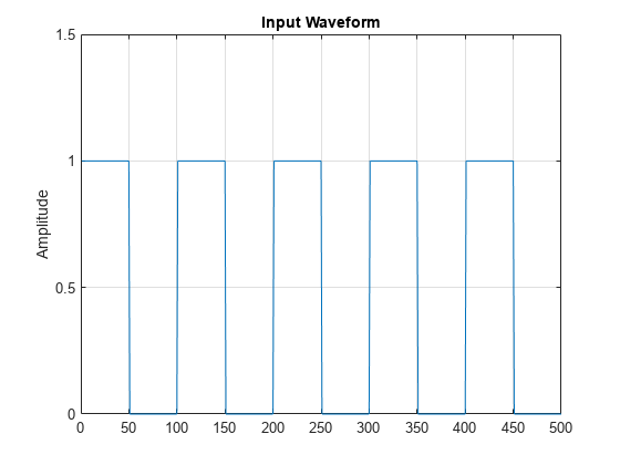
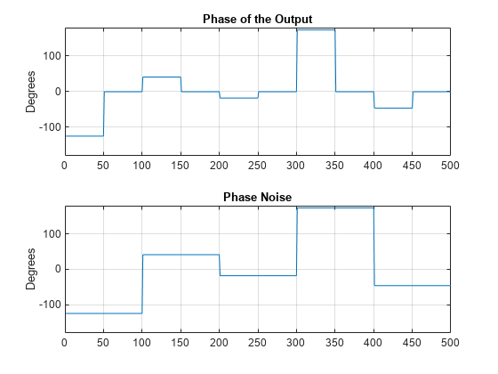
This example illustrates adding phase noise to a rectangular pulse waveform having five pulses. A random phase is added to each sample of the waveform. Compute the phase of the output waveform and compare the phase to the phase noise returned when executing the System object™.

For convenience, set the gain of the transmitter to 0 dB, the peak power to 1 W, and seed the random number generator to ensure reproducible results.

waveform = phased.RectangularWaveform('NumPulses',5);
transmitter = phased.Transmitter('CoherentOnTransmit',false,...
   'PhaseNoiseOutputPort',true,'Gain',0,'PeakPower',1,...
   'SeedSource','Property','Seed',1000);
wf = waveform();
[txtoutput,phnoise] = transmitter(wf);
phdeg = rad2deg(phnoise);
phdeg(phdeg>180)= phdeg(phdeg>180) - 360;
plot(wf)
title('Input Waveform')
axis([0 length(wf) 0 1.5])
ylabel('Amplitude')
grid on

Figure contains an axes object. The axes object with title Input Waveform, ylabel Amplitude contains an object of type line.

subplot(2,1,1)
plot(rad2deg(atan2(imag(txtoutput),real(txtoutput))))
title('Phase of the Output')
ylabel('Degrees')
axis([0 length(wf) -180 180])
grid on
subplot(2,1,2)
plot(phdeg)
title('Phase Noise'); ylabel('Degrees')
axis([0 length(wf) -180 180])
grid on

Figure contains 2 axes objects. Axes object 1 with title Phase of the Output, ylabel Degrees contains an object of type line. Axes object 2 with title Phase Noise, ylabel Degrees contains an object of type line.

The first figure shows the waveform. The phase of each pulse at the input to the transmitter is zero. In the second figure, the top plot shows the phase of the transmitter output waveform. The bottom plot shows the phase added to each sample. Focus on the first 100 samples. The pulse waveform is equal to 1 for samples 1-50 and 0 for samples 51-100. The added random phase is a constant -124.7° for samples 1-100, but this affects the output only when the pulse waveform is nonzero. In the output waveform, you see that the output waveform has a phase of -124.7° for samples 1-50 and 0 for samples 51-100. Examining the transmitter output and phase noise for samples where the input waveform is nonzero, you can see that the phase output the System object and the phase of the transmitter output agree.