Scene Visualization for Phased Array System Simulation
This example shows how to use scenario viewer to visualize a system level simulation.
Introduction
A phased array system simulation often includes many moving objects. For example, both the array and the targets can be in motion. In addition, each moving object may have its own orientations, so the bookkeeping becomes more and more challenging when more players present in the simulation.
Phased Array System Toolbox™ provides a scenario viewer to help visualize how radars and targets are moving in space. Through the scenario viewer, one can follow the trajectory of each moving platform and examine the relative motion between the radar and the target.
Visualize Trajectories
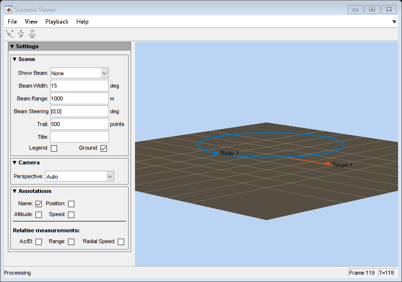
In the first example, the scenario viewer is used to visualize the trajectories of a radar and a target. Assume that the radar is circling around the origin at 3 km away. The plane with radar flies at 250 m/s (about 560 mph), and makes a circle approximately every 60 seconds.
v = 250;
deltaPhi = 360/60;
sensormotion = phased.Platform(...
    'InitialPosition',[0;-3000;500],...
    'VelocitySource','Input port',...
    'InitialVelocity',[0;v;0]);
The target is traveling along a straight road with a velocity of 30 m/s along the x-axis, which is approximately 67 mph.
tgtmotion = phased.Platform('InitialPosition',[0;0;0],...
    'Velocity',[30;0;0]);
The viewer is set to update at every 0.1 second. For the simplest case, the beam is not shown in the viewer.
tau = 0.5;
sceneview = phased.ScenarioViewer('ShowBeam','None');
This code simulates and displays radar and target's trajectories.
for m = 1:tau:60
    [sensorpos,sensorvel] = sensormotion(tau,...
        v*[cosd(m*deltaPhi);sind(m*deltaPhi);0]);
    [tgtpos,tgtvel] = tgtmotion(tau);
    sceneview(sensorpos,sensorvel,tgtpos,tgtvel);
    drawnow;
end

Visualize Trajectories and Radar Beams
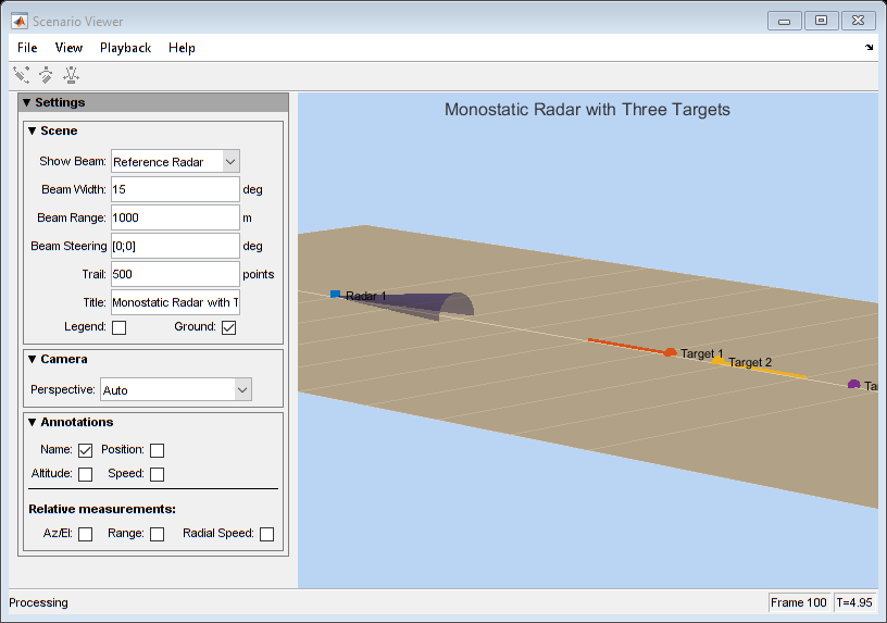
The next natural step is to visualize the antenna array beams together with the trajectories in the viewer. The following example shows how to visualize two radars and three targets moving in space. In particular, the first radar has a beam tracking the first target.
First, setup radars and targets. Note the first radar and the first target match what used in the previous section.
sensormotion = phased.Platform(...
    'InitialPosition',[0 0;-3000 500;500 1], ...
    'VelocitySource','Input port', ...
    'InitialVelocity',[0 100;v 0;0 0], ...
    'OrientationAxesOutputPort', true);
tgtmotion = phased.Platform(...
    'InitialPosition',[0 2000.66 3532.63;0 0 500;0 500 500],...
    'Velocity',[30 120 -120; 0 0 -20; 0 0 60],...
    'OrientationAxesOutputPort', true);
To properly point the beam, the scenario viewer needs to know the orientation information of radars and targets. Such information can be obtained from these moving platforms by setting the OrientationAxesOutputPort property to true at each simulation step, as shown in the code above. To pass this information to the viewer, set the scenario viewer's OrientationInputPort property to true.
sceneview = phased.ScenarioViewer('BeamRange',[3e3 3e3],...
    'BeamWidth',[5 5], ...
    'ShowBeam', 'All', ...
    'CameraPerspective', 'Custom', ...
    'CameraPosition', [-15453.85 -19716.96 13539], ...
    'CameraOrientation', [-47 -27 0]', ...
    'CameraViewAngle', 11.28, ...
    'OrientationInputPort', true, ...
    'UpdateRate',1/tau);
Note the displayed beam has a beamwidth of 5 degrees and a length of 3 km. The camera perspective is also adjusted to visualize all trajectories more clearly.
for m = 1:60
    [sensorpos,sensorvel,sensoraxis] = sensormotion(tau,...
        [v*[cosd(m*deltaPhi);sind(m*deltaPhi);0] [100; 0; 0]]);
    [tgtpos,tgtvel,tgtaxis] = tgtmotion(tau);
    % Radar 1 tracks Target 1
    [lclrng, lclang] = rangeangle(tgtpos(:,1),sensorpos(:,1),...
        sensoraxis(:,:,1));
    % Update beam direction
    sceneview.BeamSteering = [lclang [0;0]];
    sceneview(sensorpos,sensorvel,sensoraxis,tgtpos,tgtvel,tgtaxis);
    drawnow;
end

System Simulation Visualization
The scenario viewer can also be combined together with other visualizations to provide more information of the system under simulation. Next example uses a scenario viewer together with a range time intensity (RTI) scope and a Doppler time intensity (DTI) scope so an engineer can examine whether the estimated ranges and range rates of targets match the ground truth.
The example uses the radar system created in the Simulating Test Signals for a Radar Receiver example.
load BasicMonostaticRadarExampleData.mat
Consider the scene where there are three targets.
fc = radiator.OperatingFrequency;
fs = waveform.SampleRate;
c = radiator.PropagationSpeed;

sensormotion = phased.Platform(...
    'InitialPosition',[0; 0; 10],...
    'Velocity',[0; 0; 0]);

target = phased.RadarTarget(...
    'MeanRCS',[1.6 2.2 1.05],...
    'OperatingFrequency',fc);
tgtmotion = phased.Platform(...
    'InitialPosition',[2000.66 3532.63 3845.04; 0 0 0;10 10 10], ...
    'Velocity',[120 -120 0; 0 0 0; 0 0 0]);

channel = phased.FreeSpace(...
    'SampleRate',fs,...
    'TwoWayPropagation',true,...
    'OperatingFrequency',fc);
Once the echo arrives at the receiver, a matched filter and a pulse integrator are used to perform the range estimation.
matchingcoeff = getMatchedFilter(waveform);
matchingdelay = size(matchingcoeff,1)-1;
matchedfilter = phased.MatchedFilter(...
    'Coefficients',matchingcoeff,...
    'GainOutputPort',true);

prf = waveform.PRF;
fast_time_grid = unigrid(0,1/fs,1/prf,'[)');
rangeGates = c*fast_time_grid/2;

lambda = c/fc;
max_range = 5000;
tvg = phased.TimeVaryingGain(...
    'RangeLoss',2*fspl(rangeGates,lambda),...
    'ReferenceLoss',2*fspl(max_range,lambda));

num_pulse_int = 10;
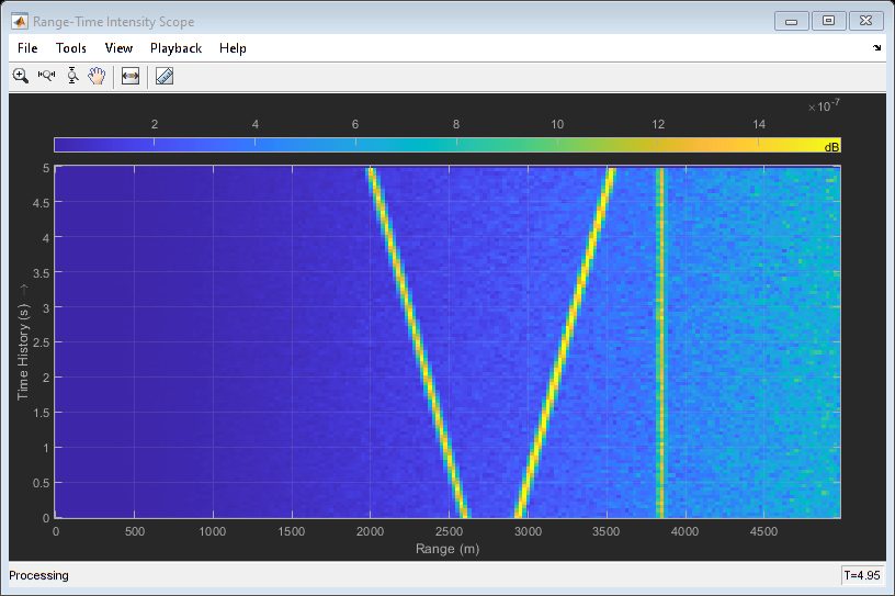
Because it is unnecessary to monitor the trajectory at the pulse repetition rate, this example assumes that the system reads the radar measurement at a rate of 20 Hz. The example uses a scenario viewer to monitor the scene and a range time intensity (RTI) plot as well as a Doppler time intensity (DTI) plot to examine the estimated range and range rate value.
r_update = 20;

sceneview = phased.ScenarioViewer('UpdateRate',r_update,...
    'Title','Monostatic Radar with Three Targets');

rtiscope = phased.IntensityScope('Name','Range-Time Intensity Scope',...
    'XLabel','Range (m)', ...
    'XResolution',c/(2*fs), ...
    'XOffset',-(matchingdelay-1)*c/(2*fs), ...
    'TimeResolution',1/r_update,'TimeSpan',5,'IntensityUnits','dB');

nfft = 128;
df = prf/nfft;
dtiscope = phased.IntensityScope(...
    'Name','Doppler-Time Intensity Scope',...
    'XLabel','Velocity (m/sec)', ...
    'XResolution',dop2speed(df,lambda)/2, ...
    'XOffset', dop2speed(-prf/2,lambda)/2, ...
    'TimeResolution',1/r_update,'TimeSpan',5,'IntensityUnits','dB');
The next section performs the system simulation and produces the visualizations.
% Pre-allocate array for improved processing speed
rxpulses = zeros(numel(rangeGates),num_pulse_int);

for k = 1:100
    for m = 1:num_pulse_int
        % Update sensor and target positions
        [sensorpos,sensorvel] = sensormotion(1/prf);
        [tgtpos,tgtvel] = tgtmotion(1/prf);

        % Calculate the target angles as seen by the sensor
        [~,tgtang] = rangeangle(tgtpos,sensorpos);

        % Simulate propagation of pulse in direction of targets
        pulse = waveform();
        [txsig,txstatus] = transmitter(pulse);
        txsig = radiator(txsig,tgtang);
        txsig = channel(txsig,sensorpos,tgtpos,sensorvel,tgtvel);

        % Reflect pulse off of targets
        tgtsig = target(txsig);

        % Receive target returns at sensor
        rxsig = collector(tgtsig,tgtang);
        rxpulses(:,m) = receiver(rxsig,~(txstatus>0));
    end

    rxpulses = matchedfilter(rxpulses);

    % Correct for matched filter delay
    rxpulses = buffer(...
        rxpulses(matchingdelay+1:end),...
        size(rxpulses,1));

    rxpulses = tvg(rxpulses);

    rx_int = pulsint(rxpulses,'noncoherent');

    % display RTI
    rtiscope(rx_int);

    % display DTI
    rx_dop = mean(fftshift(...
        abs(fft(rxpulses,nfft,2)),2));
    dtiscope(rx_dop.');

    % display scene
    sceneview(sensorpos,sensorvel,tgtpos,tgtvel);

    % perform next detection when next update is needed
    sensormotion(1/r_update);
    tgtmotion(1/r_update);
end

hide(dtiscope);
hide(rtiscope);

hide(sceneview);
show(rtiscope);

Both the scenario viewer and the RTI are updated during the simulation so one can easily verify whether the simulation is running as expected and whether the range estimation matches the ground truth while the simulation is running.
hide(rtiscope);
show(dtiscope);

Similarly, the DTI provides the range rate estimates of each target.
Conclusions
This example describes different ways to visualize the radar and target's trajectories. Such visualizations help provide an overall picture of the system dynamics.