Color Point Clouds by Point Properties

Download Data

Download a lidar tile from the USGS 3DEP NC Phase 2 survey covering downtown Wilson, North Carolina [1].

dataDir = fullfile(tempdir,"pcviewerComputedColorData");
if ~exist(dataDir,"dir")
    mkdir(dataDir)
end
ncURL = "https://rockyweb.usgs.gov/vdelivery/Datasets/Staged/" + ...
    "Elevation/LPC/Projects/NC_Phase2_2014/NC_WilsonCo_2014/LAZ/" + ...
    "USGS_LPC_NC_Phase2_2014_LA_37_20372101_.laz";
ncFile = fullfile(dataDir,"wilsonDowntown.laz");
if ~exist(ncFile,"file")
    websave(ncFile, ncURL);
end

Read Point Cloud and Remove Noise

Read the point cloud using lasFileReader and readPointCloud with classification attributes, then remove noise points (ASPRS classes 7 and 18).

readerNC = lasFileReader(ncFile);
[ptCloud, attr] = readPointCloud(readerNC, Attributes="Classification");
classLabels = attr.Classification;
noiseClasses = [7, 18];
keepIdx = ~ismember(classLabels, noiseClasses);
ptCloudClean = select(ptCloud, keepIdx);

Color by Point Density

Compute Local Density

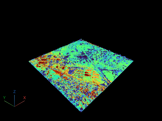
For each point, find its K nearest neighbors using findNearestNeighbors. The distance to the farthest neighbor defines the radius of a sphere enclosing those K points. Density is $$K/((4/3)\pi r^3)$$. Dense areas (flat ground, building walls) produce a small sphere and high density. Sparse areas (vegetation canopy, terrain edges) produce a large sphere and low density.

K = 30;
[~, dists] = findNearestNeighbors(ptCloudClean,ptCloudClean.Location,K+1);
dists = dists(2:end, :);
maxDist = dists(end, :)';
density = K ./ ((4/3) * pi * maxDist.^3);

Map to Colors and Visualize

Clamp outliers at the 95th percentile to spread the colormap across the meaningful range, then map to turbo. Warm colors (yellow/red) indicate high density, cool colors (blue) indicate low density.

densityClamped = density;
pHigh = prctile(density, 95);
densityClamped(densityClamped > pHigh) = pHigh;
nColors = 256;
cmap = turbo(nColors);
colorIdx = round(rescale(densityClamped, 1, nColors));
colors = cmap(colorIdx, :);
pcviewer(ptCloudClean, colors);

Color by Curvature

Compute Surface Curvature

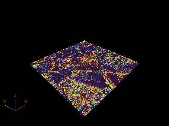
Surface curvature measures how much the local neighborhood deviates from a flat plane. For each point, perform PCA on its K nearest neighbors. The ratio $${\lambda }_{min}/\sum \lambda$$ gives the curvature: near zero for flat surfaces, larger at edges, corners, and ridges.

K = 30;
loc = double(ptCloudClean.Location);
idx = findNearestNeighbors(ptCloudClean, loc, K);
nPts = ptCloudClean.Count;
curvature = zeros(nPts, 1);
for i = 1:nPts
    neighbors = loc(idx(:,i), :);
    centered = neighbors - mean(neighbors);
    C = (centered' * centered) / K;
    eigVals = eig(C);
    curvature(i) = eigVals(1) / sum(eigVals);
end

Map to Colors and Visualize

Clamp at the 95th percentile and map to turbo. Blue indicates flat surfaces (ground, rooftops), red/yellow indicates high curvature (building edges, roof ridges, curbs).

curvClamped = curvature;
pHighCurv = prctile(curvature, 95);
curvClamped(curvClamped > pHighCurv) = pHighCurv;
colorIdx = round(rescale(curvClamped, 1, nColors));
colors = cmap(colorIdx, :);
pcviewer(ptCloudClean, colors);

Color by Distance to Ground

Compute Distance to Ground Surface

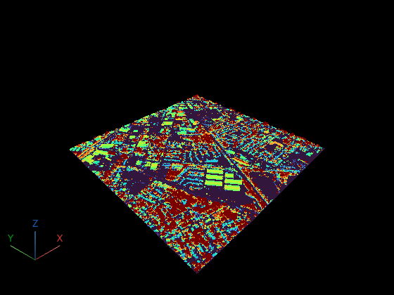
Use the classified ground points (ASPRS class 2) as a reference surface. Compute the height above the nearest ground point using pcdistance. This reveals the height of vegetation canopy, building roofs, and other above-ground structures.

ptCloudGround = readPointCloud(readerNC, Classification=2);
[~, indices] = pcdistance(ptCloudClean, ptCloudGround);
groundZ = ptCloudGround.Location(indices, 3);
distToGround = abs(double(ptCloudClean.Location(:,3)) - double(groundZ));

Map to Colors and Visualize

Clamp at the 95th percentile and map to turbo. Blue indicates points near the ground, red/yellow indicates points far above ground (treetops, rooftops).

distClamped = double(distToGround);
pHighDist = prctile(distClamped, 95);
distClamped(distClamped > pHighDist) = pHighDist;
colorIdx = round(rescale(distClamped, 1, nColors));
colors = cmap(colorIdx, :);
pcviewer(ptCloudClean, colors);

Color by Laser Return Number

Read Return Number

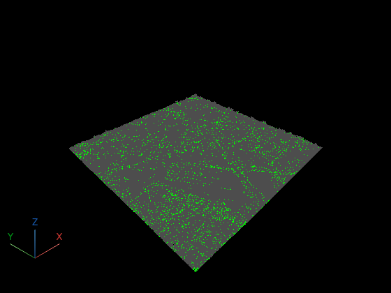
LAS/LAZ files store per-point attributes recorded during acquisition. The laser return number indicates the order in which a pulse was reflected. First returns come from the highest surface (canopy tops, roofs), while later returns penetrate through vegetation to lower surfaces. Highlighting multi-return points reveals where the laser penetrated canopy.

[~, attrReturn] = readPointCloud(readerNC, Attributes="LaserReturn");
returnNum = attrReturn.LaserReturn;
returnNumClean = returnNum(keepIdx);

Map to Colors and Visualize

Color first returns dark gray and all multi-returns (2nd, 3rd, 4th) green. Multi-return areas correspond to vegetation canopy where the laser penetrates multiple layers.

colors = repmat([0.3 0.3 0.3], ptCloudClean.Count, 1);
colors(returnNumClean > 1, :) = repmat([0.0 1.0 0.0], sum(returnNumClean > 1), 1);
pcviewer(ptCloudClean, colors);

Color by Scan Angle

Read Scan Angle

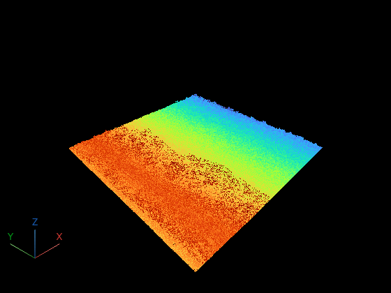
Scan angle is another per-point attribute stored in LAS/LAZ files. It is the angle of the laser beam relative to nadir (straight down). The scanner sweeps side to side as the aircraft flies, creating a swath. Points at 0 degrees are directly below the aircraft, while points at the maximum angle (±18 degrees in this dataset) are at the swath edge.

[~, attrScan] = readPointCloud(readerNC, Attributes="ScanAngle");
scanAngle = attrScan.ScanAngle;
scanAngleClean = scanAngle(keepIdx);

Map to Colors and Visualize

Map the scan angle range to turbo. Blue indicates points scanned at the left edge of the swath (negative angles), red indicates the right edge (positive angles), and green/yellow corresponds to points near nadir (center of the swath).

colorIdx = round(rescale(double(scanAngleClean), 1, nColors));
colors = cmap(colorIdx, :);
pcviewer(ptCloudClean, colors);

Blend RGB with Elevation

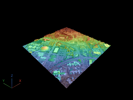
Blending RGB with an elevation gradient lets you keep visual context (recognizable trees, buildings, roads) while simultaneously emphasizing 3D structure through height variation.

Download Data

Download a second lidar tile from the Wasatch Fault survey [2]. This tile has photo-realistic RGB color and varied terrain, making it suitable for demonstrating color blending.

utahURL = "https://rockyweb.usgs.gov/vdelivery/Datasets/Staged/" + ...
    "Elevation/LPC/Projects/Wasatch_Fault_UT_LiDAR/UT_Wasatch_L4_2013/" + ...
    "LAZ/USGS_LPC_Wasatch_Fault_UT_LiDAR_12TVL2900012000.laz";
utahFile = fullfile(dataDir,"wasatchCampus.laz");
if ~exist(utahFile,"file")
    websave(utahFile, utahURL);
end
readerUtah = lasFileReader(utahFile);
ptCloudUtah = readPointCloud(readerUtah);

Remove High Outliers

A few noise points at extreme heights compress the colormap. Remove points above the 99th percentile of Z.

z = double(ptCloudUtah.Location(:,3));
ptCloudUtah = select(ptCloudUtah, z <= prctile(z, 99));

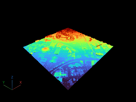
Elevation Gradient

Normalize elevation to [0,1] using the 1st and 99th percentiles, then map through turbo.

z = double(ptCloudUtah.Location(:,3));
zLow = prctile(z, 1);
zHigh = prctile(z, 99);
zNorm = max(min((z - zLow) / (zHigh - zLow), 1), 0);
elevColorIdx = round(rescale(zNorm, 1, 256));
elevColors = turbo(256);
elevColors = elevColors(elevColorIdx, :);
pcviewer(ptCloudUtah, elevColors);

Blend with RGB

Mix 50% of the original photo color with 50% of the elevation tint. The result preserves recognizable features (trees, buildings, roads) while showing height variation.

rgb = double(ptCloudUtah.Color) / 65535;
alpha = 0.5;
blended = alpha * rgb + (1 - alpha) * elevColors;
blended = min(blended, 1);
pcviewer(ptCloudUtah, blended);

References

[1] USGS Lidar Point Cloud NC_Phase2_2014 courtesy of the U.S. Geological Survey.

[2] USGS Lidar Point Cloud UT_Wasatch_L4_2013 courtesy of the U.S. Geological Survey.