Color Point Clouds in pcviewer

Download Data

Download a lidar tile from the USGS 3DEP Wasatch Fault survey [1]. This tile covers foothills near Salt Lake City, Utah and includes RGB, intensity, and classification attributes. Read it using lasFileReader and readPointCloud.

tileURL = "https://rockyweb.usgs.gov/vdelivery/Datasets/Staged/" + ...
    "Elevation/LPC/Projects/Wasatch_Fault_UT_LiDAR/UT_Wasatch_L4_2013/" + ...
    "LAZ/USGS_LPC_Wasatch_Fault_UT_LiDAR_12TVL3000012000.laz";
dataDir = fullfile(tempdir,"pcviewerColorData");
if ~exist(dataDir,"dir")
    mkdir(dataDir)
end
localFile = fullfile(dataDir,"wasatchFoothills.laz");
if ~exist(localFile,"file")
    websave(localFile, tileURL);
end
reader = lasFileReader(localFile);
ptCloud = readPointCloud(reader);

Default Color Selection

When you do not specify a color source, pcviewer automatically picks the best available attribute in this order: RGB color, then intensity, then Z elevation. This means you can visualize any point cloud without additional setup.

This point cloud has RGB, so pcviewer uses it by default.

pcviewer(ptCloud);

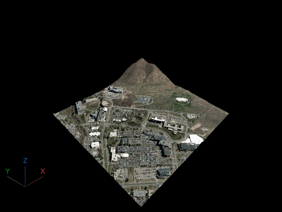
Create a version without RGB. pcviewer falls back to intensity coloring.

ptCloudIntensity = pointCloud(ptCloud.Location, Intensity=ptCloud.Intensity);
pcviewer(ptCloudIntensity);

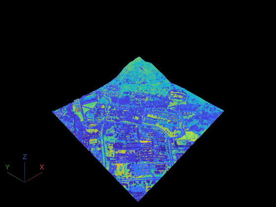
With no color or intensity, pcviewer falls back to Z elevation coloring.

ptCloudXYZ = pointCloud(ptCloud.Location);
pcviewer(ptCloudXYZ);

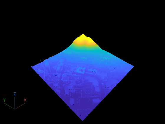
Switch Color Source

The ColorSource argument lets you switch which attribute drives the coloring without computing anything yourself. You can inspect different properties of the same data (X, Y, Z, Intensity, Color) by changing a single parameter.

viewer = pcviewer(ptCloud, ColorSource="X");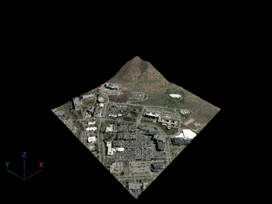

You can also change the color source on an existing viewer through the Points property, without opening a new window.

viewer = pcviewer(ptCloud, ColorSource="X");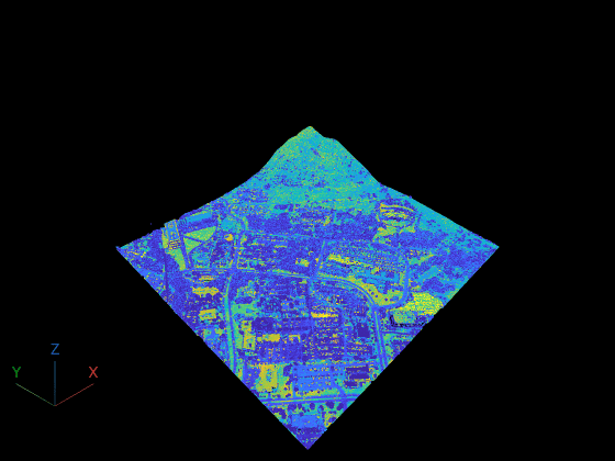

viewer.Points.ColorSource = "Intensity";

Map Scalar Values to Colors

When you compute a per-point scalar from any analysis, you can map it to an M-by-3 RGB array through a colormap and pass it directly to pcviewer. This lets you visualize any derived quantity (density, curvature, distance) on the point cloud.

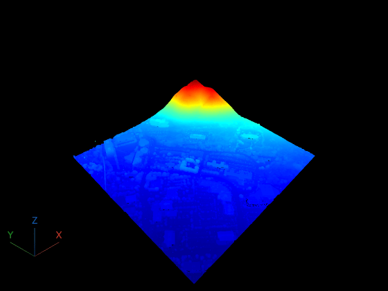
As an example, map elevation values through the jet colormap to create a height gradient.

zValues = ptCloud.Location(:,3);
cmap = jet(256);
colorIdx = round(rescale(zValues, 1, 256));
colors = cmap(colorIdx, :);
pcviewer(ptCloud, colors);

Overlay Multiple Point Clouds

Use addPointCloud to overlay additional point clouds in a single viewer, each with its own color array. This is useful for comparing datasets, highlighting subsets, or visualizing segmentation results in context.

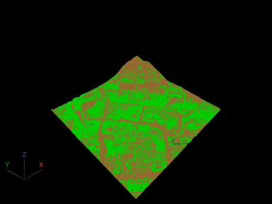
Here, segment the ground using segmentGroundSMRF and display it in brown, then overlay the non-ground points in green.

groundIdx = segmentGroundSMRF(ptCloud);
ptCloudGround = select(ptCloud, groundIdx);
ptCloudNonGround = select(ptCloud, ~groundIdx);
groundColor = repmat([0.6 0.4 0.2], ptCloudGround.Count, 1); % brown
nonGroundColor = repmat([0 0.8 0], ptCloudNonGround.Count, 1); % green
viewer = pcviewer(ptCloudGround, groundColor);

viewer.addPointCloud(ptCloudNonGround, nonGroundColor);

Color by Cluster Labels

Crop the non-ground points to a 200 m x 200 m area and cluster them using pcsegdist. Assign each cluster a distinct color from hsv.

roi = [430000 430200 4512400 4512600 -inf inf];
ptCloudCropped = select(ptCloudNonGround, findPointsInROI(ptCloudNonGround, roi));
minDistance = 2; % meters
minClusterPoints = 2000;
[labels, numClusters] = pcsegdist(ptCloudCropped, minDistance, NumClusterPoints=minClusterPoints);
cmap = hsv(numClusters);
colors = zeros(ptCloudCropped.Count, 3);
validIdx = labels > 0;
colors(validIdx,:) = cmap(labels(validIdx),:);
pcviewer(ptCloudCropped, colors);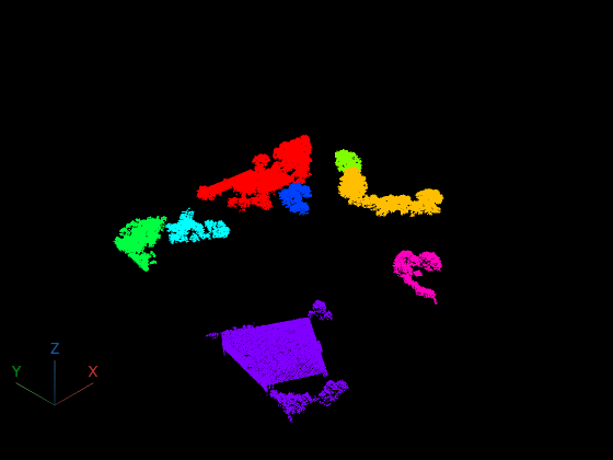

References

[1] USGS Lidar Point Cloud UT_Wasatch_L4_2013 courtesy of the U.S. Geological Survey.