Lidar Extrinsic Calibration Using Ground Plane

Overview

A lidar sensor mounted on a vehicle measures the 3-D world in its own coordinate frame. For downstream algorithms, such as obstacle detection, free-space estimation, mapping, and sensor fusion, to work correctly, you must know how the sensor frame of the mounted lidar sensor relates to the vehicle body frame. Six extrinsic parameters describe the relationship: three translational (X, Y, and Z) and three rotational (roll, pitch, and yaw).

Traditional extrinsic calibration requires placing a known target, such as a checkerboard or retroreflective panel, in a controlled environment. This method is impractical for fleets of autonomous vehicles, agricultural equipment operating in the field, or robots deployed across many facilities. A practical approach uses the ground, which is always available.

By fitting a plane to the ground surface in a single lidar scan, you can recover three of the six extrinsic parameters:

This figure shows the extrinsic parameters, together with an example vehicle coordinate system and the plane normal.

lidarExtrinsicsIllustration

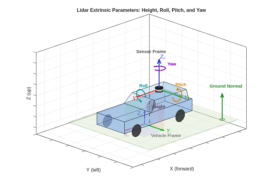
The ground plane does not provide yaw (rotation around the Z-axis) because a flat surface appears unchanged when rotated about its normal. To estimate yaw, you must use a different technique, such as comparing lidar-derived motion with known vehicle motion along a straight path.

This example estimates extrinsic parameters using these steps:

Load Point Cloud Data

Load a point cloud captured by an Ouster® OS-1 64-beam lidar sensor into the workspace. The scan was captured in an indoor office environment with cubicles on a flat floor, and includes a partial view of the ceiling, providing a suitable scenario for ground-plane calibration. The same technique applies to outdoor scenes such as roads, parking lots, agricultural fields, and other predominantly flat surfaces.

Because the plane-fitting step uses RANSAC, a randomized algorithm, set the random number seed to ensure repeatable results.

rng(0)

ptCloud = pcread("officeOuster64.pcd");

figure
pcshow(ptCloud)
xlabel("X")
ylabel("Y")
zlabel("Z");
title("Original Point Cloud")

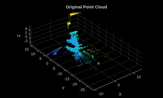
The raw scan contains the full lidar field of view. The scene includes the floor, walls, ceiling, furniture, and other objects. Ground points are mixed with other points. To improve plane fitting, reduce the search space by cropping the point cloud.

Crop Point Cloud to Region of Interest

A lidar scan can extend tens of meters in all directions. Points far from the sensor are sparser and noisier. Distant surfaces such as walls and parked vehicles can reduce plane-fitting accuracy. To focus the analysis on nearby ground points, crop the point cloud to a cylindrical region around the sensor where point density is highest and the flat-ground assumption is most reliable.

To focus on nearby ground points, choose a crop radius that captures a sufficient area of the floor while excluding most walls and distant clutter. For this indoor scan, you can use a radius of 4 meters. For outdoor, vehicle-mounted lidar data, you can use a larger radius depending on terrain flatness.

cropRadius = 4; % meters
idx = ptCloud.findPointsInCylinder(cropRadius,VerticalAxis="X");
ptCloud = ptCloud.select(idx);

figure
pcshow(ptCloud)
xlabel("X")
ylabel("Y")
zlabel("Z")
title("Cropped Point Cloud (4 m Cylinder)")

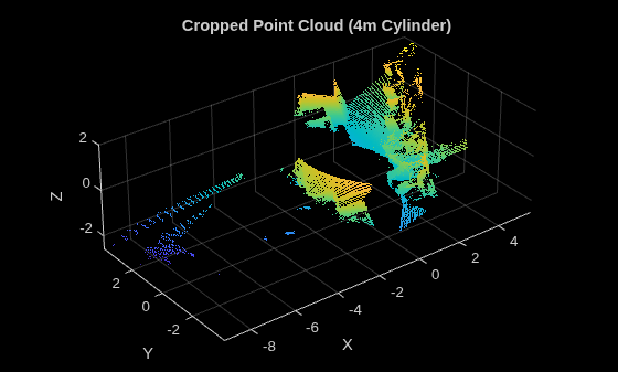
After cropping, the floor becomes the dominant flat surface in the scene, which can improve plane-fitting accuracy.

Fit Ground Plane of Point Cloud Using RANSAC

The function pcfitplane uses the Random Sample Consensus (RANSAC) algorithm to find the dominant plane in the point cloud. RANSAC repeatedly selects small random subsets of points, fits a plane to each subset, and counts the number of points close to each plane. The algorithm selects the plane with the most inliers as the dominant plane.

The fit depends primarily on these parameters:

Fit a plane to the cropped point cloud.

maxDistance = 0.06; % meters
[planeMdl,inlierIdx,outlierIdx] = pcfitplane(ptCloud,maxDistance, ...
    MaxNumTrials=10000,Confidence=97);

The result is a planeModel object that contains the plane equation $$ax+by+cz+d=0$$, where $$[abc]$$ is the unit normal vector. To verify the fit, visualize the inliers (ground points) and outliers (other points).

groundPts    = select(ptCloud,inlierIdx);
nonGroundPts = select(ptCloud,outlierIdx);

figure
pcshow(groundPts.Location,"blue")
hold on
pcshow(nonGroundPts.Location,"red")
xlabel("X")
ylabel("Y")
zlabel("Z")
title("Ground Inliers (Blue) and Outliers (Red)")

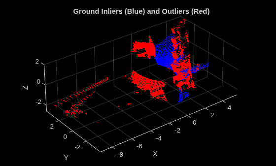
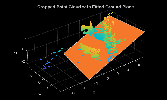
Overlay the fitted plane model on the point cloud to verify alignment with the floor points. The overlaid plane coincides with the floor point subset.

figure
pcshow(ptCloud)
hold on
plot(planeMdl)
xlabel("X")
ylabel("Y")
zlabel("Z");
title("Cropped Point Cloud with Fitted Ground Plane")

Estimate Sensor Mounting Height

The sensor mounting height is the perpendicular distance from the sensor, located at the coordinate origin, to the fitted ground plane. For a plane $$ax+by+cz+d=0$$, the distance from the origin is:

$$ h = abs(d)/sqrt(a^2 + b^2 + c^2) $$

If the pcfitplane function returns a unit normal, the denominator equals 1 and the height simplifies to $$|d|$$. This code estimates sensor height using the general formula to ensure robustness.

abcd = planeMdl.Parameters;
height = abs(abcd(4))/norm(abcd(1:3));
fprintf("Estimated sensor height: %.3f m\n",height)

Estimated sensor height: 0.940 m

Estimate Pitch and Roll of Sensor

A plane normal vector has two angular degrees of freedom. You can represent the plane normal as a point on the unit sphere. When the sensor is level, the ground-plane normal points straight up in the sensor frame: [0 0 1]. Any deviation from vertical reveals sensor tilt:

The normalRotation function computes the rigid rotation that aligns the fitted ground-plane normal with the reference vertical direction [0 0 1]. This rotation represents the sensor pitch and roll expressed in the vehicle frame.

Before computing the rotation, ensure that the normal points upward (positive Z-component). If the normal points downward, flip the plane parameters to avoid a 180-degree ambiguity.

% Ensure the normal points upward
n = planeMdl.Normal;
if n(3) < 0
    planeMdl = planeModel(-planeMdl.Parameters);
end

% Compute the rotation that aligns the ground normal to [0 0 1]
tform = normalRotation(planeMdl,[0 0 1]);

Extract Euler angles from the resulting transform. Using the XYZ convention, the first angle represents roll and the second angle represents pitch. You cannot derive the third angle, yaw, from the ground plane alone.

eulAngles = rad2deg(se3(tform).eul("XYZ"));

roll  = eulAngles(1);
pitch = eulAngles(2);

fprintf("Height: %.3f m | Pitch: %.2f° | Roll: %.2f°\n",height,pitch,roll)

Height: 0.940 m | Pitch: 22.85° | Roll: 4.19°

Apply Correction to Point Cloud and Visualize

Apply the estimated rotation to the original cropped point cloud. This transforms the data from the tilted sensor frame into a level vehicle frame where the ground is flat and horizontal. This corrected point cloud serves as the input to downstream perception algorithms.

correctedCloud = pctransform(ptCloud,tform);

figure
pcshow(correctedCloud)
xlabel("X")
ylabel("Y")
zlabel("Z")
title("Corrected Point Cloud (Ground Leveled)")

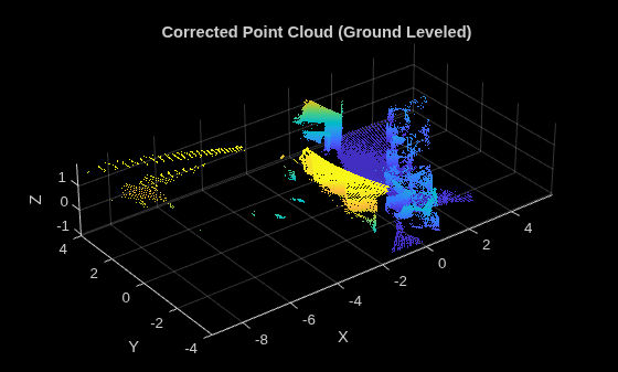
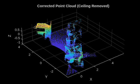
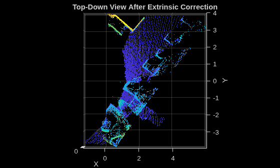
For a cleaner view, remove points above the sensor height (ceiling) and behind the sensor. Then, display a top-down view of the point cloud. Occupancy grids, path planning, and obstacle maps commonly use this perspective. In the adjusted view, the office cubicles and a wall appear more clearly.

xValBehindLidar = -2;
keepIdx = (correctedCloud.Location(:,3) < height) & ...
          (correctedCloud.Location(:,1) > xValBehindLidar);
correctedCloud = correctedCloud.select(keepIdx);

figure
pcshow(correctedCloud)
xlabel("X")
ylabel("Y")
zlabel("Z")
title("Corrected Point Cloud (Ceiling Removed)")

figure
pcshow(correctedCloud,ViewPlane="XY")
xlabel("X")
ylabel("Y")
title("Top-Down View After Extrinsic Correction")

Summary

In this example, you learned a target-free method for recovering three lidar extrinsic parameters (height, pitch, and roll) from a single point cloud by fitting the ground plane.

To complete a full 6-DOF extrinsic calibration, estimate yaw separately, for example by comparing lidar-derived ego-motion against a known heading over a straight-line drive segment.