Point Cloud to Surface Mesh for RF Propagation Analysis

Load and Inspect the Point Cloud

Read the boardroom point cloud captured by a 3-D scanner. The scan contains over 25 million points with color and position data. Download the "Boardroom" lidar scan (merged & resampled, 0.4 GB) in PLY format from the Indoor Lidar-RGBD Scan Dataset page.

pc = pcread("boardroom.ply");
pcview = pcviewer(pc);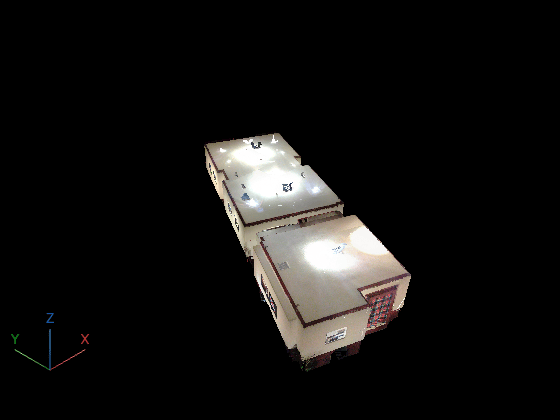

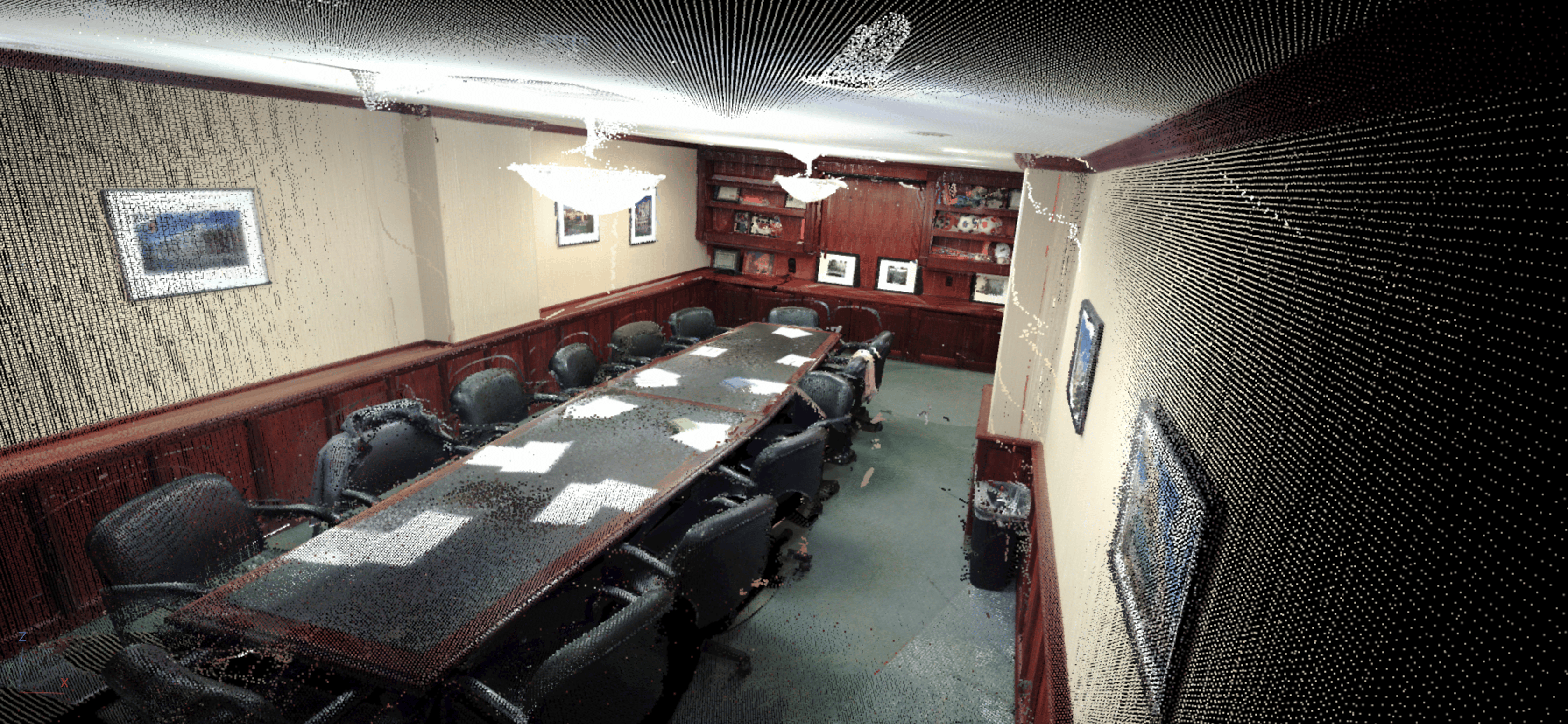
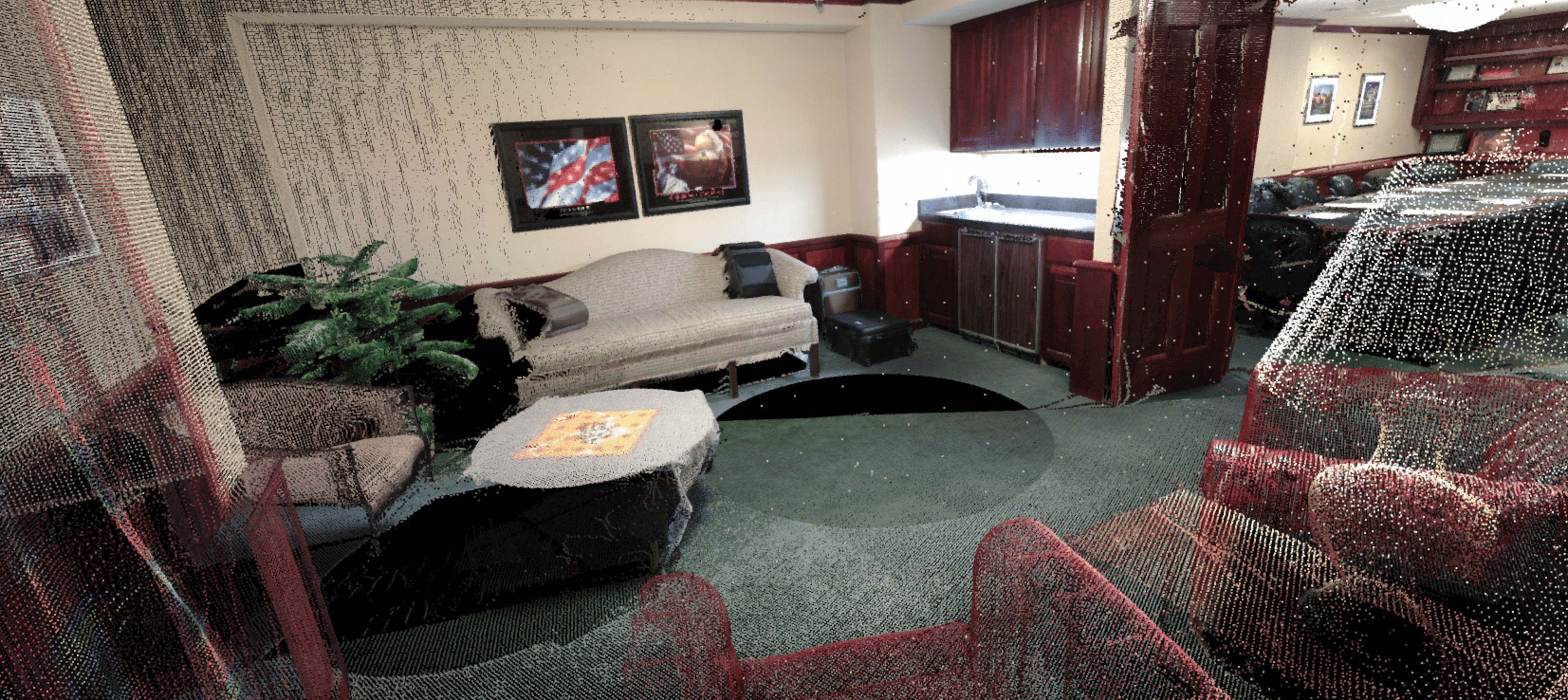
View of the point cloud by using pcviewer controls to zoom, rotate and pan.

Downsample the Point Cloud

Downsample the point cloud. This significantly reduces the computation time for mesh reconstruction while preserving the overall room geometry.

pcDown = pcdownsample(pc, "gridAverage", 0.02);
pcdownview = pcviewer(pcDown);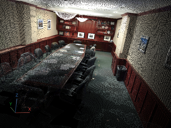

pcdownview.CameraPosition = [-0.7379 -1.1368 66.9148];
pcdownview.CameraTarget = [4.6784 13.4776 61.0893];
pcdownview.CameraUpVector = [-0.1774 -0.2082 0.9619];

Clear Point Cloud Normals

Clear any existing normals so that pc2surfacemesh computes consistent normals internally during Poisson reconstruction.

pcDown.Normal = [];

Reconstruct Surface Mesh Using Poisson Method

Use pc2surfacemesh to create a watertight surface mesh from the downsampled point cloud using Poisson reconstruction.

tic
mesh = pc2surfacemesh(pcDown, "poisson");
toc

Elapsed time is 7.608393 seconds.

Visualize the Reconstructed Mesh

meshview = pcviewer();

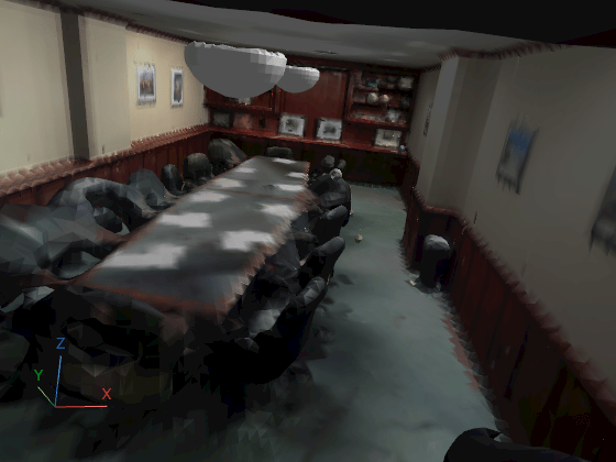
meshview.addSurfaceMesh(mesh);
meshview.CameraPosition = [-0.7379 -1.1368 66.9148];
meshview.CameraTarget = [4.6784 13.4776 61.0893];
meshview.CameraUpVector = [-0.1774 -0.2082 0.9619];

Export Mesh as STL

Write the surface mesh to an STL file. Site Viewer can load STL files directly as 3-D scene models.

stlFile = "boardroom_mesh.stl";
writeSurfaceMesh(mesh, stlFile);

Launch Site Viewer with the Boardroom Mesh

Create a Site Viewer using the STL file as the 3-D scene model. Specifying SceneModel automatically sets cartesian coordinate system.

viewer = siteviewer(SceneModel=stlFile, ShowEdges="off");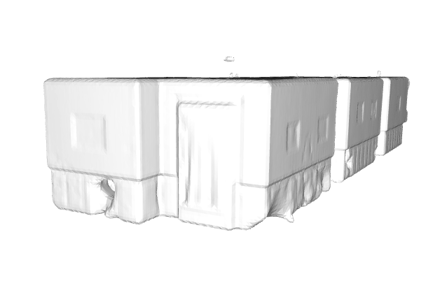

Adjust Face Normals for Interior Viewing

Site Viewer performs backface culling based on face normals. Poisson reconstruction produces outward-facing normals, which causes interior walls to appear invisible when viewing from inside the room. To fix this, reverse the face winding order by swapping the second and third vertex indices in each triangle. This flips the normals inward so interior surfaces render correctly.

viewer.close();
tri = triangulation(double(mesh.Faces(:,[1 3 2])), mesh.Vertices);
viewer = siteviewer(SceneModel=tri, ShowEdges="off");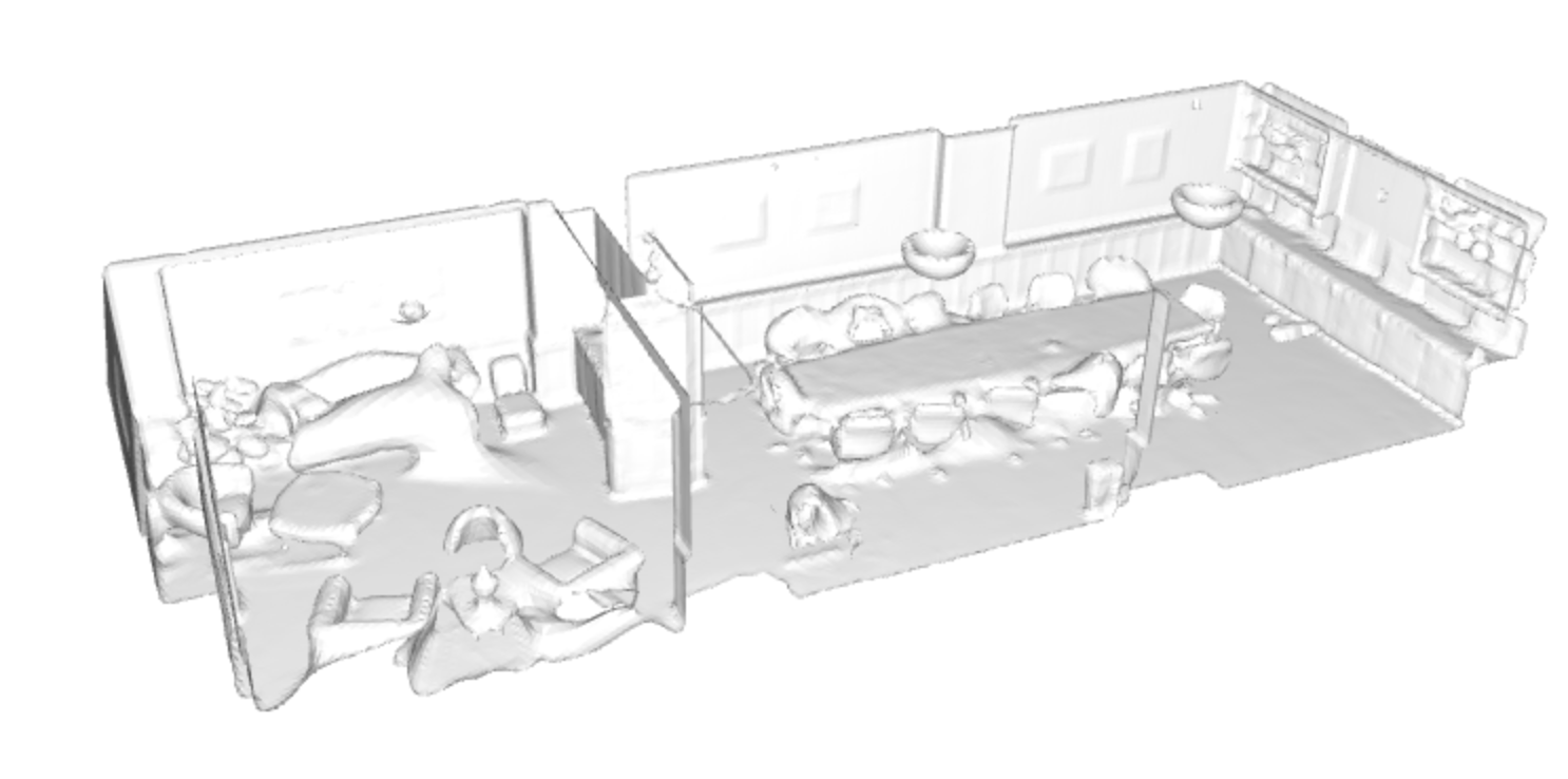

Create Transmitter and Receiver Sites

Place a WiFi access point (5.8 GHz) as the transmitter near the ceiling and multiple receivers at various locations representing devices on tables and shelves throughout the room.

tx = txsite("cartesian", ...
    AntennaPosition=[-2; 2; 66.7], ...
    TransmitterFrequency=5.8e9);
rx1 = rxsite("cartesian", AntennaPosition=[-0.3571; 1.1271; 65.6921]);
rx2 = rxsite("cartesian", AntennaPosition=[-0.0415; 5.5482; 64.9562]);
rx3 = rxsite("cartesian", AntennaPosition=[2.8801; 6.6349; 65.7364]);
rx4 = rxsite("cartesian", AntennaPosition=[-4.0225; -2.6860; 65.4973]);
rx5 = rxsite("cartesian", AntennaPosition=[-1.4037; -3.8992; 65.3961]);
rx = [rx1 rx2 rx3 rx4 rx5];
show(tx, ShowAntennaHeight=false)
show(rx, ShowAntennaHeight=false)

Compute Line-of-Sight Visibility

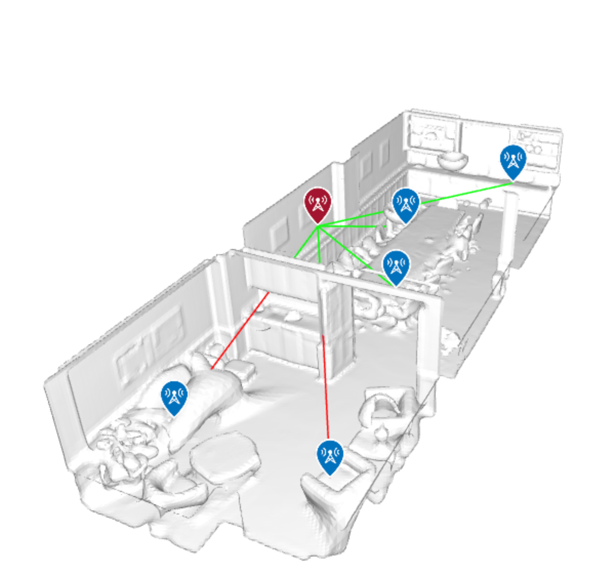
Before running ray tracing, check which receivers have a direct line of sight to the transmitter. The reconstructed mesh determines which paths are obstructed by walls or furniture.

los(tx, rx)

Perform Ray Tracing Analysis

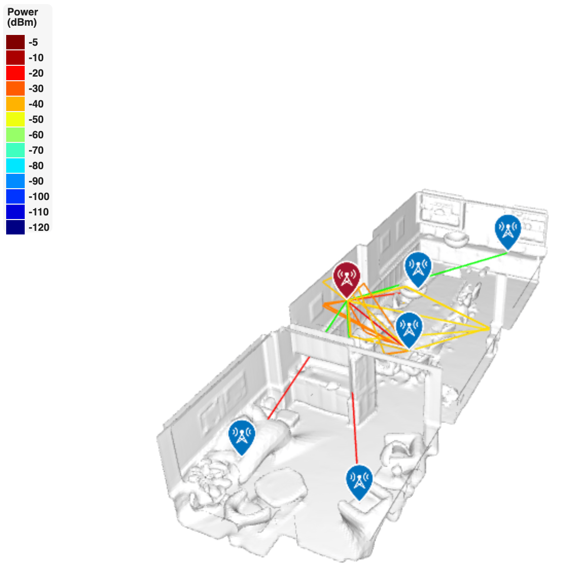
Create a ray tracing propagation model using the SBR (shooting and bouncing rays) method. With default settings, the model traces direct paths between the transmitter and receivers.

pm = propagationModel("raytracing", ...
    CoordinateSystem="cartesian");
raytrace(tx, rx, pm)

Ray Tracing with Reflections

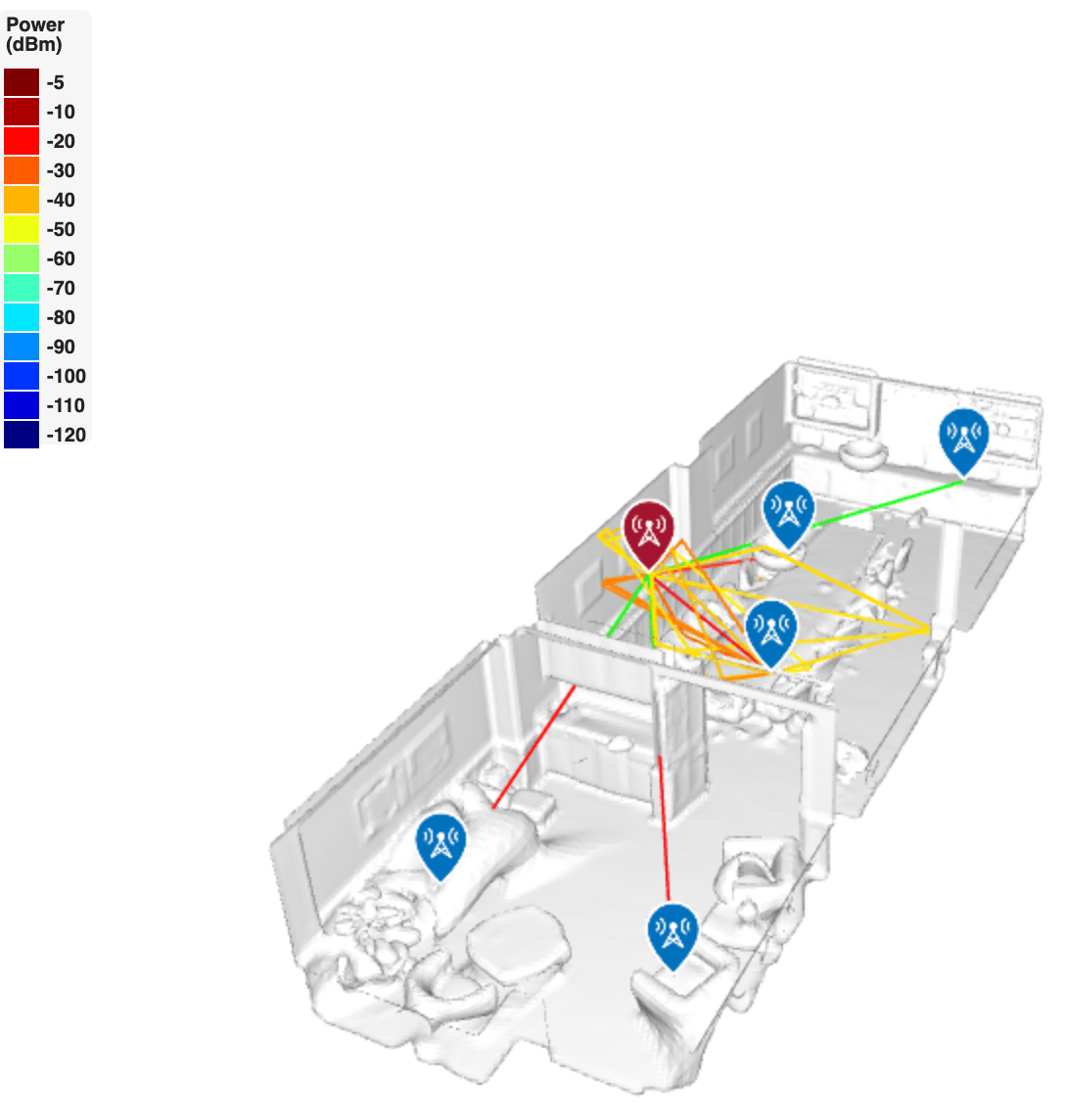
Increase the maximum number of reflections to 3 to capture additional propagation paths that bounce off walls, floor, and ceiling. This reveals how signals reach receivers that may not have a direct line of sight.

pm.MaxNumReflections = 3;
raytrace(tx, rx, pm)

Compute and Display Signal Strength

Calculate received signal strength at each receiver location using the ray tracing model with reflections.

ss = sigstrength(rx, tx, pm);
for idx = 1:numel(ss)
    disp("Receiver " + idx + " signal strength: " + ss(idx) + " dBm")
end

Receiver 1 signal strength: -10.4543 dBm
Receiver 2 signal strength: -19.4316 dBm
Receiver 3 signal strength: -Inf dBm
Receiver 4 signal strength: -Inf dBm
Receiver 5 signal strength: -Inf dBm