NoiseAnomaly
Description
Add-On Required: This feature requires the Time Series Anomaly Detection for MATLAB add-on.
The NoiseAnomaly object specifies the characteristics of an
additive noise anomaly model that you can inject into a time series using injectAnomaly.
Name-value argument specifications in injectAnomaly determine the window
location and length during which the anomaly occurs.
You create this model using syntheticAnomaly. NoiseAnomaly is one type of anomaly model in
a set of anomaly objects that you can use to perturb a time series in multiple ways. You can
then use this perturbed time series to help validate anomaly detection models against
different anomaly types.
For an example of creating a synthetic anomaly object, see Create and Inject Synthetic Anomaly Models
Properties
Object Functions
injectAnomaly | Inject anomalies defined by one or more anomaly models into a univariate time series |
Examples
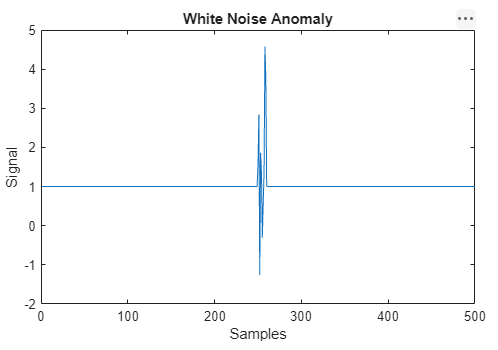
Create a NoiseAnomaly model that models white noise that has a standard deviation and a mean of 3.0.
noiseanom = syntheticAnomaly("Noise",Type="White",Std=3,Mean = 3.0);
Create a "StuckAtConstant" model that sticks at a custom constant of 1.5.
sacanom = syntheticAnomaly("StuckAtConstant",Type="Custom",Value=1.5);
Combine the anomalies into a vector so that they can be injected together into a time series.
anomvec = [noiseanom sacanom]
anomvec =
1×2 AnomalyTypes:

 NoiseAnomaly, StuckAtConstantAnomaly
Load and plot the healthy single-variable time series channel1, which serves as the injection target.
load HealthySineWaveU channel1
Plot the time series.
plot(channel1)
title("Healthy Time Series")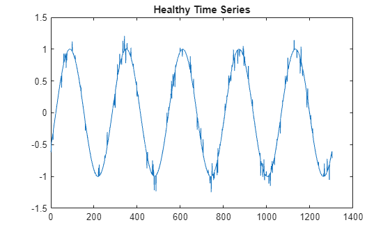
Inject the anomalies into channel1. For example repeatability, specify starting positions for the two anomalies.
[channel1_anom,labels] = injectAnomaly(anomvec,channel1,WindowStart=[185 1080]);
The resulting signal is channel1_anom. The labels output identifies where the anomalies are injected.
ianom = find(labels==1);
ianom(1:8)
ans = 8×1

   185
   186
   187
   188
   189
   190
   191
   192
plot(channel1_anom)
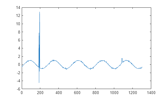
The anomalies appear where WindowStart specifies.
Version History
Introduced in R2026a