Detect Abrupt System Changes Using Identification Techniques
This example shows how to detect abrupt changes in the behavior of a system using online estimation and automatic data segmentation techniques. This example uses functionality from System Identification Toolbox™, and does not require Predictive Maintenance Toolbox™.
Problem Description
Consider a linear system whose transport delay changes from two to one second. Transport delay is the time taken for the input to affect the measured output. In this example, you detect the change in transport delay using online estimation and data segmentation techniques. Input-output data measured from the system is available in the data file pdmAbruptChangesData.mat.
Load and plot the data.
load pdmAbruptChangesData.mat
z = iddata(z(:,1),z(:,2));
plot(z)
grid on
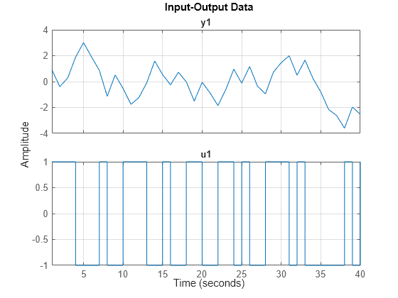
The transport delay change takes place around 20 seconds, but is not easy to see in the plot.
Model the system using an ARX structure with one A polynomial coefficient, two B polynomial coefficients, and one delay.
Here, A = [1 a] and B = [0 b1 b2].
The leading coefficient of the B polynomial is zero because the model has no feedthrough. As the system dynamics change, the values of the three coefficients a, b1, and b2 change. When b1 is close to zero, the effective transport delay will be 2 samples because the B polynomial has 2 leading zeros. When b1 is larger, the effective transport delay will be 1 sample.
Thus, to detect changes in transport delay you can monitor changes in the B polynomial coefficients.
Use Online Estimation for Change Detection
Online estimation algorithms update model parameters and state estimates in a recursive manner, as new data becomes available. You can perform online estimation using Simulink blocks from the System Identification Toolbox library or at the command line using recursive identification routines such as recursiveARX. Online estimation can be used to model time varying dynamics such as aging machinery and changing weather patterns, or to detect faults in electromechanical systems.
As the estimator updates the model parameters, a change in system dynamics (delay) will be indicated by a larger than usual change in the values of the parameters b1 and b2. Changes in the B polynomial coefficients will be tracked by computing:
Use the recursiveARX object for online parameter estimation of the ARX model.
na = 1;
nb = 2;
nk = 1;
Estimator = recursiveARX([na nb nk]);
Specify the recursive estimation algorithm as NormalizedGradient and the adaptation gain as 0.9.
Estimator.EstimationMethod = 'NormalizedGradient';
Estimator.AdaptationGain = .9;
Extract the raw data from the iddata object, z.
Output = z.OutputData;
Input = z.InputData;
t = z.SamplingInstants;
N = length(t);
Use animated lines to plot the estimated parameter values and L. Initialize these animated lines prior to estimation. To simulate streaming data, feed the data to the estimator one sample at a time. Initialize the model parameters before estimation, and then perform online estimation.
%% Initialize plot
Colors = {'r','g','b'};
fig = figure;
ax = axes(fig);
for k = 3:-1:1
   h(k) = animatedline('Color',Colors{k}); % lines for a, b1 and b2 parameters
end
h(4) =  animatedline('Marker','.','Color',[0 0 0]); % line for L
legend({'a','b1','b2','Deviation'},'location','southeast')
title('ARX Recursive Parameter Estimation')
xlabel('Time (seconds)')
ylabel('Parameter value')
ax.XLim = [t(1),t(end)];
ax.YLim = [-2, 2];
grid on
box on

%% Now perform recursive estimation and show results
n0 = 6;
L = NaN(N,nk);
B_old = NaN(1,3);
for ct = 1:N
   [A,B] = step(Estimator,Output(ct),Input(ct));
   if ct>n0
      L(ct) = norm(B-B_old);
      B_old = B;
   end
   addpoints(h(1),t(ct),A(2))
   addpoints(h(2),t(ct),B(2))
   addpoints(h(3),t(ct),B(3))
   addpoints(h(4),t(ct),L(ct))
   pause(0.1)
end
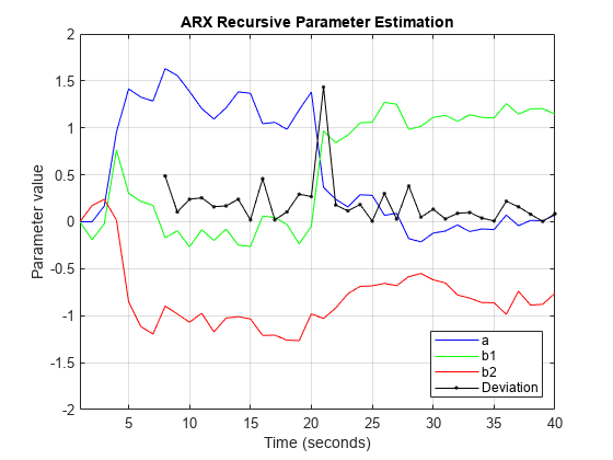
The first n0 = 6 samples of the data are not used for computing the change-detector, L. During this interval the parameter changes are large owing to the unknown initial conditions.
Find the location of all peaks in L by using the findpeaks command from Signal Processing Toolbox.
[v,Loc] = findpeaks(L);
[~,I] = max(v);
line(t(Loc(I)),L(Loc(I)),'parent',ax,'Marker','o','MarkerEdgeColor','r',...
   'MarkerFaceColor','y','MarkerSize',12)
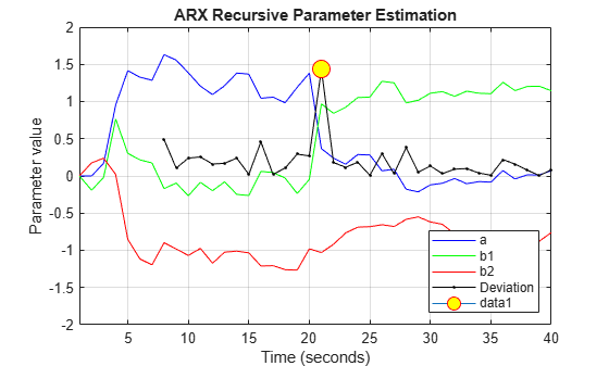
fprintf('Change in system delay detected at sample number %d.\n',Loc(I));Change in system delay detected at sample number 21.
The location of the largest peak corresponds to the largest change in the B polynomial coefficients, and is thus the location of a change in transport delay.
While online estimation techniques provide more options for choosing estimation methods and model structure, the data segmentation method can help automate detection of abrupt and isolated changes.
Use Data Segmentation for Change Detection
A data segmentation algorithm automatically segments the data into regions of different dynamic behavior. This is useful for capturing abrupt changes arising from a failure or change of operating conditions. The segment command facilitates this operation for single-output data. segment is an alternative to online estimation techniques when you do not need to capture the time-varying behavior during system operation.
Applications of data segmentation include segmentation of speech signals (each segment corresponds to a phoneme), failure detection (the segments correspond to operation with and without failures), and estimation of different working modes of a system.
Inputs to the segment command include the measured data, the model orders, and a guess for the variance, r2, of the noise that affects the system. If the variance is entirely unknown, it can be estimated automatically. Perform data segmentation using an ARX model of the same orders as used for online estimation. Set the variance to 0.1.
[seg,V,tvmod] = segment(z,[na nb nk],0.1);
The method for segmentation is based on AFMM (adaptive forgetting through multiple models). For details about the method, see Andersson, Int. J. Control Nov 1985.
A multi-model approach is used to track the time-varying system. The resulting tracking model is an average of the multiple models and is returned as the third output argument of segment, tvmod.
Plot the parameters of the tracking model.
plot(tvmod)
legend({'a','b_1','b_2'},'Location','best')
xlabel('Samples'), ylabel('Parameter value')
title('Time-varying estimates')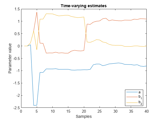
Note the similarity between these parameter trajectories and those estimated using recursiveARX.
segment determines the time points when changes have occurred using tvmod and q, the probability that a model exhibits abrupt changes. These time points are used to construct the segmented model by employing a smoothing procedure over the tracking model.
The parameter values of the segmented model are returned in seg, the first output argument of segment. The values in each successive row are the parameter values of the underlying segmented model at the corresponding time instants. These values remain constant over successive rows and change only when the system dynamics are determined to have changed. Thus, values in seg are piecewise constant.
Plot the estimated values for parameters a, b1, and b2.
plot(seg)
title('Parameter value segments')
legend({'a','b1','b2'},'Location','best')
xlabel('Time (seconds)')
ylabel('Parameter value')
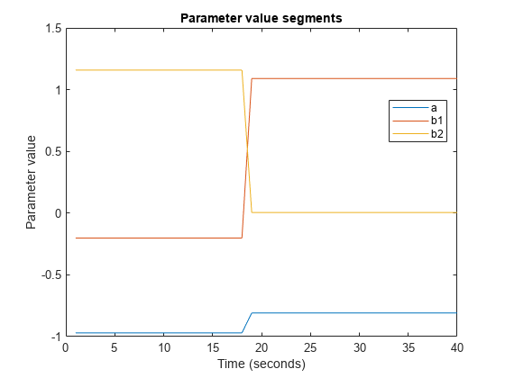
A change is seen in the parameter values around sample number 19. The value of b1 changes from a small (close to zero) to large (close to 1) value. The value of b2 shows the opposite pattern. This change in the values of the B parameters indicates a change in the transport delay.
The second output argument of segment, V, is the loss function for the segmented model (i.e. the estimated prediction error variance for the segmented model). You can use V to assess the quality of the segmented model.
Note that the two most important inputs for the segmentation algorithm are r2 and q, the fourth input argument to segment. In this example, q was not specified because the default value, 0.01, was adequate. A smaller value of r2 and a larger value of q will result in more segmentation points. To find appropriate values, you can vary r2 and q and use the ones that work the best. Typically, the segmentation algorithm is more sensitive to r2 than q.
Conclusions
The use of online estimation and data segmentation techniques for detecting abrupt changes in system dynamics was evaluated. Online estimation techniques offer more flexibility and more control over the estimation process. However, for changes that are infrequent or abrupt, segment facilitates an automatic detection technique based on smoothing of time-varying parameter estimates.