Apply Generated MATLAB Function to Expanded Data Set

Load Data and Create Reduced Data Set

Load the data set pumpData. pumpData is a 240-member ensemble table that contains simulated measurements for flow and pressure. pumpData also contains categorical fault codes that represent combinations of three independent faults. For example, a fault code of 0 represents data from a system with no faults. A fault code of 111 represents data from a system with all three faults.

load savedPumpData pumpData

View a histogram of original fault codes. The histogram shows the number of ensemble members associated with each fault code.

fcCat = pumpData{:,3};
histogram(fcCat)
title('Fault Code Distribution for Full Pump Data Set')
xlabel('Fault Codes')
ylabel('Number of Members')

Create a subset of this data set that contains 10% of the data, or 24 members. Because simulation data is often clustered, generate a randomized index with which to select the members. For the purposes of this example, first use rng to create a repeatable random seed.

rng('default')

Compute a randomized 24-element index vector idx. Sort the vector so that the indices are in order.

pdh = height(pumpData);
nsel = 24;
idx = randi(pdh,nsel,1);
idx = sort(idx);

Use idx to select member rows from pumpData.

pdSub = pumpData(idx,:);

View a histogram of the fault codes in the reduced data set.

fcCatSub = pdSub{:,3};
histogram(fcCatSub)
title('Fault Code Distribution for Reduced Pump Data Set')
xlabel('Fault Codes')
ylabel('Number of Members')

All the fault combinations are represented.

Import Reduced Data Set into Diagnostic Feature Designer

Open Diagnostic Feature Designer by using the diagnosticFeatureDesigner command. Import pdSub into the app.

Extract Time-Domain Features

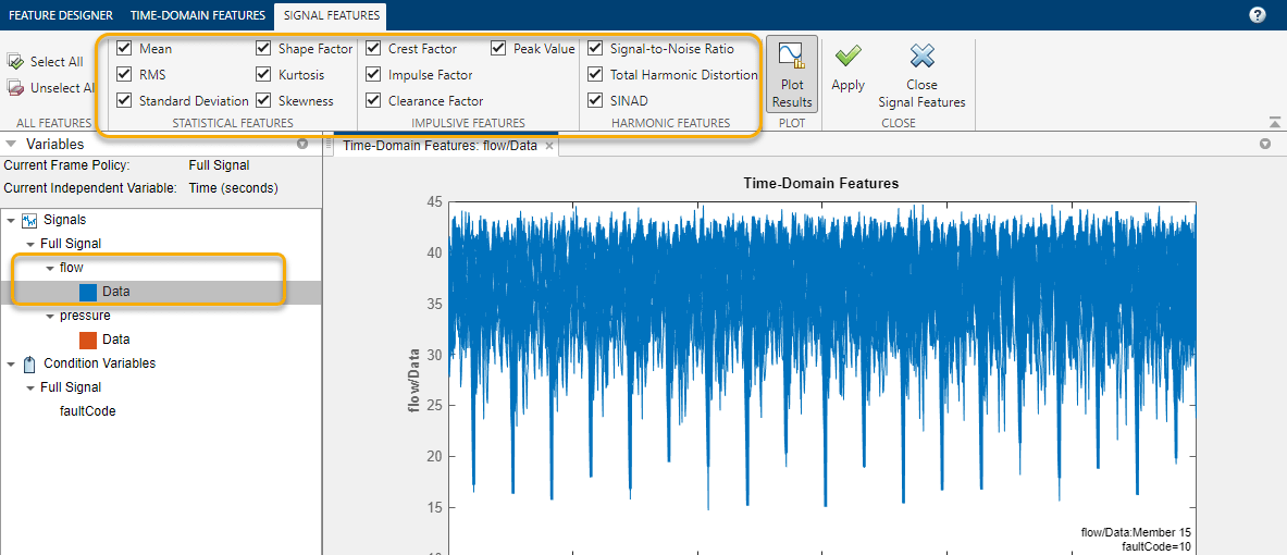
Extract the time-domain signal features from both the flow and pressure signals. For each signal, first, select the signal. Then, in the Feature Designer tab, select Time Domain Features > Signal Features and select all features.

Extract Frequency Domain Features

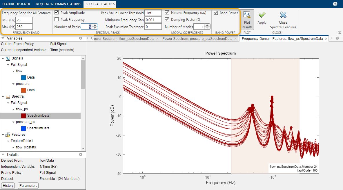
As Analyze and Select Features for Pump Diagnostics describes, computing the frequency spectrum of the flow highlights the cyclic nature of the flow signal. Estimate the frequency spectrum by selecting Spectral Estimation > Autoregressive model and using the options shown for both flow and pressure.

From the derived flow and pressure spectra, compute spectral features in the band 23–250 Hz, using the options shown.

Rank Features

Rank your features by selecting Rank Features > FeatureTable1. Because faultCode contains multiple possible values, the app defaults to the One-Way ANOVA ranking method.

Export Features to Classification Learner

Export the features set to Classification Learner so that you can train a classification model. In the Feature Ranking tab, click Export > Export Features to the Classification Learner. Select the top 15 features by selecting Select top features and typing 15.

Train Models in Classification Learner

Once you click Export, Classification Learner opens a new session using the data you exported. Start the session by clicking Start Session.

Train all available models by clicking All in the Classification Learner tab, and then Train All.

Classification Learner trains all the models and initially sorts then by name. Use the Sort by menu to sort by Accuracy (Validation). For this session, the highest scoring model, KNN, has an accuracy of about 63%. Your results may vary. Click Confusion Matrix to view the confusion matrix for this model.

Generate Code to Compute Feature Set

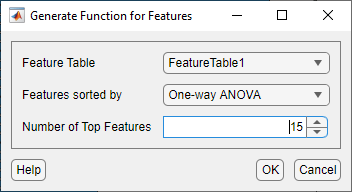
Now that you have completed your interactive feature work with a small data set, you can apply the same computations to the full data set using generated code. In Diagnostic Feature Designer, generate a function to calculate the features. To do so, in the Feature Ranking Tab, select Export > Generate Function for Features. Select the same 15 features that you exported to Classification Learner.

When you click OK, a function appears in the editor.

Save the function to your local folder as diagnosticFeatures.

Apply the Function to Full Data Set

Execute diagnosticFeatures with the full pumpData ensemble to get the 240-member feature set. Use the following command.

feature240 = diagnosticFeatures(pumpData);

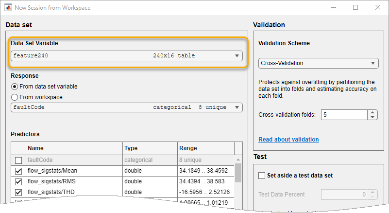
feature240 is a 240-by-16 table. The table includes the condition variable faultCode and the 15 features.

Train Models in Classification Learner with Larger Feature Table

Train classification models again in Classification Learner, using feature240 this time. Open a new session window using the following command.

classificationLearner

In the Classification Learner window, click New Session > From Workspace. In the New Session window, in Data Set > Data Set Variable, select feature240.

Repeat the steps you performed with the 24-member data set. Start the session and then train all models. Sort the models by Accuracy (Validation). In this session, the highest scoring model is Bagged Trees, with an accuracy of about 73%, roughly 10% higher than the model computed using the reduced data. Again, your results may vary, but they should still reflect the increase in best accuracy

For this session, the highest model accuracy, achieved by both Bagged Trees and RUSBoosted Trees, is around 80%. Again, your results may vary, but they should still reflect the increase in best accuracy.