Condition Monitoring and Prognostics Using Vibration Signals

Data Description

Load vibration data stored in pdmBearingConditionMonitoringData.mat (this is a large dataset ~88MB that is downloaded from the MathWorks support files site). The data is stored in a cell array, which was generated using a ball bearing signal simulator with single point defect on the outer race of the bearing. It contains multiple segments of vibration signals for bearings simulated in different health conditions (defect depth increases from 3um to above 3mm). Each segment stores signals collected for 1 second at a sampling rate of 20 kHz. In pdmBearingConditionMonitoringData.mat, the defectDepthVec stores how defect depth changes versus time while the expTime stores the corresponding time in minutes.

url = 'https://www.mathworks.com/supportfiles/predmaint/condition-monitoring-and-prognostics-using-vibration-signals/pdmBearingConditionMonitoringData.mat';
websave('pdmBearingConditionMonitoringData.mat',url);
load pdmBearingConditionMonitoringData.mat

% Define the number of data points to be processed.
numSamples = length(data);

% Define sampling frequency.
fs = 20E3;          % unit: Hz

Plot how defect depth changes in different segments of data.

plot(expTime,defectDepthVec);
xlabel('Time (min)');
ylabel('Defect depth (m)');

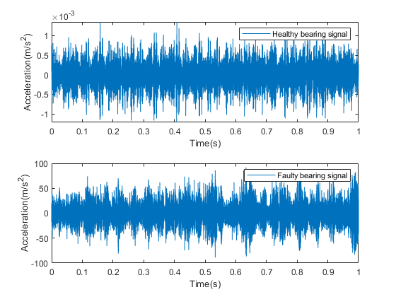
Plot the healthy and faulty data.

time = linspace(0,1,fs)';

% healthy bearing signal
subplot(2,1,1);
plot(time,data{1});
xlabel('Time(s)');
ylabel('Acceleration(m/s^2)');
legend('Healthy bearing signal');

% faulty bearing signal
subplot(2,1,2);
plot(time,data{end});
xlabel('Time(s)');
ylabel('Acceleration(m/s^2)');
legend('Faulty bearing signal');

Feature Extraction

In this section, representative features are extracted from each segment of data. These features will be used for health monitoring and prognostics. Typical features for bearing diagnostics and prognostics include time-domain features (root mean square, peak value, signal kurtosis, etc.) or frequency-domain features (peak frequency, mean frequency, etc.).

Before selecting which features to use, plot the vibration signals spectrogram. Visualizing signals in time-domain or frequency-domain or time-frequency domain can help discover signal patterns that indicate degradation or failure.

First calculate the spectrogram of the healthy bearing data. Use a window size of 500 data points and an overlap ratio of 90% (equivalent to 450 data points). Set the number of points for the FFT to be 512. fs represents the sampling frequency defined previously.

[~,fvec,tvec,P0] = spectrogram(data{1},500,450,512,fs);

P0 is the spectrogram, fvec is the frequency vector and tvec is the time vector.

Plot the spectrogram of the healthy bearing signal.

clf;
imagesc(tvec,fvec,P0)
xlabel('Time(s)');
ylabel('Frequency(Hz)');
title('Healthy Bearing Signal Spectrogram');
axis xy

Now plot the spectrogram of vibration signals that have developed faulty patterns. You can see that signal energies are concentrated at higher frequencies.

[~,fvec,tvec,Pfinal] = spectrogram(data{end},500,450,512,fs);
imagesc(tvec,fvec,Pfinal)
xlabel('Time(s)');
ylabel('Frequency(Hz)');
title('Faulty Bearing Signal Spectrogram');
axis xy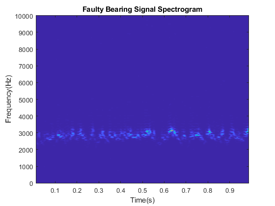

Since the spectrograms for data from healthy and faulty bearings are different, representative features can be extracted from spectrograms and used for condition monitoring and prognostics. In this example, extract mean peak frequencies from spectrograms as health indicators. Denote the spectrogram as $$P(t,\omega )$$. Peak frequency at each time instance is defined as:

The mean peak frequency is the average of peak frequencies defined above.

Calculate the mean peak frequency for healthy ball bearing signals.

[~,I0] = max(P0);               % Find out where the peak frequencies are located.
meanPeakFreq0 = mean(fvec(I0))  % Calculate mean peak frequency.

meanPeakFreq0 = 666.4602

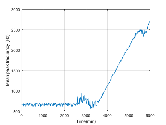
The healthy bearing vibration signals have mean peak frequency at around 650 Hz. Now calculate the mean peak frequency for faulty bearing signals. The mean peak frequency shifts to above 2500 Hz.

[~,Ifinal] = max(Pfinal);
meanPeakFreqFinal = mean(fvec(Ifinal))

meanPeakFreqFinal = 2.8068e+03

Examine the data at middle stage, when the defect depth is not very large but starting to affect the vibration signals.

[~,fvec,tvec,Pmiddle] = spectrogram(data{end/2},500,450,512,fs);
imagesc(tvec,fvec,Pmiddle)
xlabel('Time(s)');
ylabel('Frequency(Hz)');
title('Bearing Signal Spectrogram');
axis xy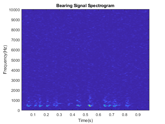

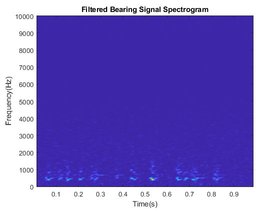
The high frequency noise components are spread all over the spectrogram. Such phenomena are mixed effects of both original vibrations and the vibrations induced by small defects. To accurately calculate mean peak frequency, filter the data to remove those high frequency components.

Apply a median filter to the vibration signals to remove high frequency noise components as well as to preserve useful information in the high frequencies.

dataMiddleFilt = medfilt1(data{end/2},3);

Plot spectrogram after median filtering. The high frequency components are suppressed.

[~,fvec,tvec,Pmiddle] = spectrogram(dataMiddleFilt,500,450,512,fs);
imagesc(tvec,fvec,Pmiddle)
xlabel('Time(s)');
ylabel('Frequency(Hz)');
title('Filtered Bearing Signal Spectrogram');
axis xy

Since the mean peak frequency successfully distinguishes healthy ball bearings from faulty ball bearings, extract mean peak frequency from each segment of data.

% Define a progress bar.
h = waitbar(0,'Start to extract features');
% Initialize a vector to store the extracted mean peak frequencies.
meanPeakFreq = zeros(numSamples,1);
for k = 1:numSamples
    % Get most up-to-date data.
    curData = data{k};
    % Apply median filter.
    curDataFilt = medfilt1(curData,3);
    % Calculate spectrogram.
    [~,fvec,tvec,P_k] = spectrogram(curDataFilt,500,450,512,fs);
    % Calculate peak frequency at each time instance.
    [~,I] = max(P_k);
    meanPeakFreq(k) = mean(fvec(I));
    % Show progress bar indicating how many samples have been processed.
    waitbar(k/numSamples,h,'Extracting features');
end
close(h);

Plot the extracted mean peak frequencies versus time.

plot(expTime,meanPeakFreq);
xlabel('Time(min)');
ylabel('Mean peak frequency (Hz)');
grid on;

Condition Monitoring and Prognostics

In this section, condition monitoring and prognostics are performed using a pre-defined threshold and dynamic models. For condition monitoring, create an alarm that triggers if the mean peak frequency exceeds the predefined threshold. For prognostics, identify a dynamic model to forecast the values of mean peak frequencies in the next few hours. Create an alarm that triggers if the forecast mean peak frequency exceeds the predefined threshold.

Forecasting helps us better prepare for a potential fault or even stop the machine before failure. Consider the mean peak frequency as a time series. We can estimate a time series model for the mean peak frequency and use the model to forecast the future values. Use the first 200 mean peak frequency values to create an initial time series model, then once 10 new values are available, use the last 100 values to update the time series model. This batch mode of updating the time series model captures instantaneous trends. The updated time series model is used to compute a 10 step ahead forecast.

tStart = 200;               % Start Time
timeSeg = 100;              % Length of data for building dynamic model
forecastLen = 10;           % Define forecast time horizon
batchSize = 10;             % Define batch size for updating the dynamic model

For prognostics and condition monitoring, you need to set a threshold to decide when to stop the machine. In this example, use the statistical data of healthy and faulty bearing generated from simulation to determine the threshold. The pdmBearingConditionMonitoringStatistics.mat stores the probability distributions of mean peak frequencies for healthy and faulty bearings. The probability distributions are computed by perturbing the defect depth of healthy and faulty bearings.

url = 'https://www.mathworks.com/supportfiles/predmaint/condition-monitoring-and-prognostics-using-vibration-signals/pdmBearingConditionMonitoringStatistics.mat';
websave('pdmBearingConditionMonitoringStatistics.mat',url);
load pdmBearingConditionMonitoringStatistics.mat

Plot the probability distributions of mean peak frequency for healthy and faulty bearings.

plot(pFreq,pNormal,'g--',pFreq,pFaulty,'r');
xlabel('Mean peak frequency(Hz)');
ylabel('Probability Distribution');
legend('Normal Bearing','Faulty Bearing');

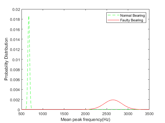
Based on this plot, set the threshold for the mean peak frequency to 2000Hz to distinguish normal bearings from faulty bearings as well as maximize the use of the bearings.

threshold = 2000;

Calculate sampling time and convert its unit to seconds.

samplingTime = 60*(expTime(2)-expTime(1));                  % unit: seconds
tsFeature = iddata(meanPeakFreq(1:tStart),[],samplingTime);

Plot the initial 200 mean peak frequency data.

plot(tsFeature.y)

The plot shows that the initial data is a combination of constant level and noise. This is expected as initially the bearing is healthy and the mean peak frequency is not expected to change significantly

Identify a second-order state-space model using the first 200 data points. Obtain the model in canonical form and specify the sampling time.

past_sys = ssest(tsFeature,2,'Ts',samplingTime,'Form','canonical')

past_sys =
  Discrete-time identified state-space model:
    x(t+Ts) = A x(t) + K e(t)
       y(t) = C x(t) + e(t)
 
  A = 
            x1       x2
   x1        0        1
   x2   0.9605  0.03942
 
  C = 
       x1  x2
   y1   1   0
 
  K = 
              y1
   x1  -0.003899
   x2   0.003656
 
Sample time: 600 seconds
  
Parameterization:
   CANONICAL form with indices: 2.
   Disturbance component: estimate
   Number of free coefficients: 4
   Use "idssdata", "getpvec", "getcov" for parameters and their uncertainties.

Status:                                               
Estimated using SSEST on time domain data "tsFeature".
Fit to estimation data: 0.2763% (prediction focus)    
FPE: 640, MSE: 602.7                                  

The initial estimated dynamic model has a low goodness of fit. The goodness of fit metric is the normalized root mean square error (NRMSE), calculated as

where $$x_{true}$$ is the true value, $$x_{pred}$$ is the predicted value.

When the estimation data is a combination of constant level and noise, $$x_{pred}\approx mean(x_{true})$$, giving a NRMSE close to 0. To validate the model, plot the autocorrelation of residuals.

resid(tsFeature,past_sys)

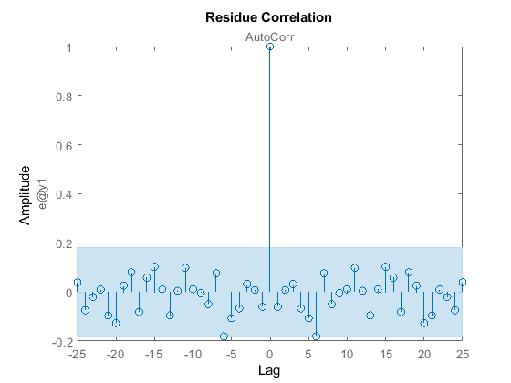
As seen, the residuals are uncorrelated and the generated model is valid.

Use the identified model past_sys to forecast mean peak frequency values and compute the standard deviation of the forecasted values.

[yF,~,~,yFSD] = forecast(past_sys,tsFeature,forecastLen);

Plot the forecasted values and confidence intervals.

tHistory = expTime(1:tStart);
forecastTimeIdx = (tStart+1):(tStart+forecastLen);
tForecast = expTime(forecastTimeIdx);

% Plot historical data, forecast value and 95% confidence interval.
plot(tHistory,meanPeakFreq(1:tStart),'b',...
     tForecast,yF.OutputData,'kx',...
     [tHistory; tForecast], threshold*ones(1,length(tHistory)+forecastLen), 'r--',...
     tForecast,yF.OutputData+1.96*yFSD,'g--',...
     tForecast,yF.OutputData-1.96*yFSD,'g--');

ylim([400, 1.1*threshold]);
ylabel('Mean peak frequency (Hz)');
xlabel('Time (min)');
legend({'Past Data', 'Forecast', 'Failure Threshold', '95% C.I'},...
    'Location','northoutside','Orientation','horizontal');
grid on;

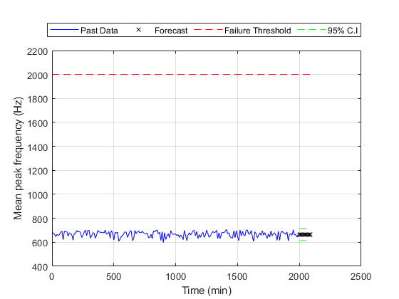
The plot shows that the forecasted values of the mean peak frequency are well below the threshold.

Now update model parameters as new data comes in, and re-estimate the forecasted values. Also create an alarm to check if the signals or the forecasted value exceed the failure threshold.

for tCur = tStart:batchSize:numSamples
    %  latest features into iddata object.
    tsFeature = iddata(meanPeakFreq((tCur-timeSeg+1):tCur),[],samplingTime);
    
    % Update system parameters when new data comes in. Use previous model
    % parameters as initial guesses.
    sys = ssest(tsFeature,past_sys);
    past_sys = sys;
    
    % Forecast the output of the updated state-space model. Also compute
    % the standard deviation of the forecasted output.
    [yF,~,~,yFSD]  = forecast(sys, tsFeature, forecastLen);
    
    % Find the time corresponding to historical data and forecasted values.
    tHistory = expTime(1:tCur);
    forecastTimeIdx = (tCur+1):(tCur+forecastLen);
    tForecast = expTime(forecastTimeIdx);
    
    % Plot historical data, forecasted mean peak frequency value and 95%
    % confidence interval.
    plot(tHistory,meanPeakFreq(1:tCur),'b',...
              tForecast,yF.OutputData,'kx',...
              [tHistory; tForecast], threshold*ones(1,length(tHistory)+forecastLen), 'r--',...
              tForecast,yF.OutputData+1.96*yFSD,'g--',...
              tForecast,yF.OutputData-1.96*yFSD,'g--');

    ylim([400, 1.1*threshold]);
    ylabel('Mean peak frequency (Hz)');
    xlabel('Time (min)');
    legend({'Past Data', 'Forecast', 'Failure Threshold', '95% C.I'},...
           'Location','northoutside','Orientation','horizontal');
    grid on;
    
    % Display an alarm when actual monitored variables or forecasted values exceed
    % failure threshold.
    if(any(meanPeakFreq(tCur-batchSize+1:tCur)>threshold))
        disp('Monitored variable exceeds failure threshold');
        break;
    elseif(any(yF.y>threshold))
        % Estimate the time when the system will reach failure threshold.
        tAlarm = tForecast(find(yF.y>threshold,1));
        disp(['Estimated to hit failure threshold in ' num2str(tAlarm-tHistory(end)) ' minutes from now.']);
        break;
    end
end

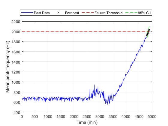
Estimated to hit failure threshold in 80 minutes from now.

Examine the most recent time series model.

sys

sys =
  Discrete-time identified state-space model:
    x(t+Ts) = A x(t) + K e(t)
       y(t) = C x(t) + e(t)
 
  A = 
           x1      x2
   x1       0       1
   x2  0.2624   0.746
 
  C = 
       x1  x2
   y1   1   0
 
  K = 
           y1
   x1  0.3902
   x2  0.3002
 
Sample time: 600 seconds
  
Parameterization:
   CANONICAL form with indices: 2.
   Disturbance component: estimate
   Number of free coefficients: 4
   Use "idssdata", "getpvec", "getcov" for parameters and their uncertainties.

Status:                                               
Estimated using SSEST on time domain data "tsFeature".
Fit to estimation data: 92.53% (prediction focus)     
FPE: 499.3, MSE: 442.7                                

The goodness of fit increases to above 90%, and the trend is correctly captured.

Conclusions

This example shows how to extract features from measured data to perform condition monitoring and prognostics. Based on extracted features, dynamic models are generated, validated and used to forecast time of failures so that actions can be taken before actual failures happen.