Data Analysis and Feature Extraction for Battery Raw Cycling Data
This example shows the workflow of organizing and analyzing raw data from battery test cyclers. The example, using batteryTestDataParser and batteryTestFeatureExtractor, focuses on extracting critical features from the data to understand Lithium-ion Batteries (LIBs) behavior and prepare for AI-based health monitoring and management systems.
Battery Cell Data
The measurements from LIBs are collected during cycling tests under fast-charging conditions, using a 48-channel Arbin LBT potentiostat within a temperature-controlled chamber set at 30°C [1]. You can access the detailed description of the dataset here [2]. This example focuses a single cell that is cycled to failure (80% state of health) in order to provide a comprehensive view of its performance over time. The cycling sequence exercises the battery cell with dynamic fast charging and constant 4C discharging. The cell data includes essential measurements and per-cycle summaries:
Date Time: Recorded in date-time format, which may be reset during a cycle due to data collection errors.
Cycle Index: An integer identifying the cycle number.
Step Index: An integer identifying the steps within the fast-charging policy.
Current: Measured in amperes (A).
Voltage: Measured in volts (V).
Temperature: Measured in degrees Celsius (°C).
Load the battery cell data from the MathWorks® support files site. To generalize across different battery cyclers, only the essential measurements specified above are utilized.
dataFile = matlab.internal.examples.downloadSupportFile("predmaint","batteryagingdata/singlecell/v1/singleCellLifeTimeData.zip");
unzip(dataFile)
load("singleCellLifeTimeData.mat")
head(data,5)
    Data_Point    Test_Time          DateTime          Step_Time    Step_Index    Cycle_Index    Current    Voltage    Charge_Capacity    Discharge_Capacity    Charge_Energy    Discharge_Energy       dV/dt       Internal_Resistance    Temperature
    __________    _________    ____________________    _________    __________    ___________    _______    _______    _______________    __________________    _____________    ________________    ___________    ___________________    ___________

        1               0      13-May-2017 03:21:40      -1780          0              0            0       3.3018            0                   0                   0                 0            -1.5259e-05         0.022012            30.457
        2          0.0001      13-May-2017 03:21:40      -1780          0              0            0       3.3018            0                   0                   0                 0            -1.5259e-05         0.022012            30.457
        3          9.9983      13-May-2017 03:21:50      -1770          0              0            0       3.3018            0                   0                   0                 0            -2.6703e-05         0.022012            30.445
        4          20.002      13-May-2017 03:22:00      -1760          0              0            0       3.3018            0                   0                   0                 0            -1.5259e-05         0.022012            30.501
        5          30.001      13-May-2017 03:22:10      -1750          0              0            0       3.3018            0                   0                   0                 0            -8.5831e-06         0.022012            30.501
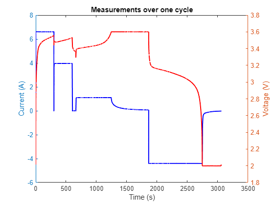
To understand the charging and discharging policy, visualize the current and voltage measurements for one cycle of the battery. In each cycle, the battery is fully charged until it reaches 3.6V and fully discharged when it reaches 2V.
cycleData = data(data.Cycle_Index == 1, :);
cycleData.DateTime = seconds(cycleData.DateTime - cycleData.DateTime(1));
figure;
yyaxis left;
plot(cycleData.DateTime,cycleData.Current, '-b', 'LineWidth', 1.5);
ylabel('Current (A)');
yyaxis right;
plot(cycleData.DateTime,cycleData.Voltage, '-r', 'LineWidth', 1.5);
ylabel('Voltage (V)');
xlabel("Time (s)");
title('Measurements over one cycle');
Data Exploration with batteryTestDataParser: Understand, Evaluate, and Prepare the Data
1. Parse and segment data
To identify the cycling phases and modes and based on the measurements, use batteryTestDataParser. This function enables raw data visualization, aids in identifying anomalies, and prepare high-quality data. Properly understanding and preparing the input data ensures its suitability for meaningful feature extraction and in-depth analysis.
Create the parser object bparser to encapsulate the data and specify the properties that correspond to the names of the variables in the data.
bParser = batteryTestDataParser(data);
bParser.CurrentVariable = 'Current';
bParser.VoltageVariable= "Voltage";
bParser.TimeVariable = "DateTime";
bParser.CycleIndexVariable = 'Cycle_Index';
bParser.StepIndexVariable = 'Step_Index';
Use segmentData to identify the cycling phase and mode that each data point belongs to, and flag invalid data points. If segmentData determines that a data point cannot be definitively assigned to a cycling phase or mode, the function marks the data point as invalid and excludes it from analysis and feature extraction. As a result, segmentData introduces three additional columns to the data in bparser: CyclingModes, CyclingPhases, and IsValid.
segmentedRawDataTable = segmentData(bParser);
head(segmentedRawDataTable,5)
    Data_Point    Test_Time          DateTime          Step_Time    Step_Index    Cycle_Index    Current    Voltage    Charge_Capacity    Discharge_Capacity    Charge_Energy    Discharge_Energy       dV/dt       Internal_Resistance    Temperature    CyclingModes    CyclingPhases    IsValid
    __________    _________    ____________________    _________    __________    ___________    _______    _______    _______________    __________________    _____________    ________________    ___________    ___________________    ___________    ____________    _____________    _______

        1               0      13-May-2017 03:21:40      -1780          0              0            0       3.3018            0                   0                   0                 0            -1.5259e-05         0.022012            30.457           Rest            Rest          true
        2          0.0001      13-May-2017 03:21:40      -1780          0              0            0       3.3018            0                   0                   0                 0            -1.5259e-05         0.022012            30.457           Rest            Rest          true
        3          9.9983      13-May-2017 03:21:50      -1770          0              0            0       3.3018            0                   0                   0                 0            -2.6703e-05         0.022012            30.445           Rest            Rest          true
        4          20.002      13-May-2017 03:22:00      -1760          0              0            0       3.3018            0                   0                   0                 0            -1.5259e-05         0.022012            30.501           Rest            Rest          true
        5          30.001      13-May-2017 03:22:10      -1750          0              0            0       3.3018            0                   0                   0                 0            -8.5831e-06         0.022012            30.501           Rest            Rest          true
Display the segmented data for chosen cycles, with each cycle divided into several segments. Each segment is associated with a specific cycling mode, denoted by a unique color.
cycleList = unique(segmentedRawDataTable(segmentedRawDataTable.IsValid, :).Cycle_Index);
maxCycle = max(cycleList);
cycleIndex = 1;
hPlotRawMeasurementsWithSegments(segmentedRawDataTable, bParser, cycleIndex)
1;
hPlotRawMeasurementsWithSegments(segmentedRawDataTable, bParser, cycleIndex)![Figure contains 2 axes objects and another object of type subplottext. Axes object 1 with xlabel Time [s], ylabel Voltage [V] contains 5 objects of type line. One or more of the lines displays its values using only markers These objects represent data, CC, CV, Rest, Undefined. Axes object 2 with xlabel Time [s], ylabel Current [A] contains 5 objects of type line. One or more of the lines displays its values using only markers These objects represent data, CC, CV, Rest, Undefined.](../../examples/predmaint/win64/BatteryCyclingDataFeatureExtractionExample_02.png)
2. Find abnormal data points
During the data collection process, time is expected to be recorded in a non-decreasing sequence with predefined time interval. However, unusually long intervals between data points might occur due to computer auto-restarts [1]. Extended periods between consecutive data points can potentially distort the temporal resolution of the dataset.
Define a long time interval as 3600 seconds. Identify any point-to-point time intervals within one cycle that exceed this duration, as they are considered abnormal.
longInterval = 3600;
timeDiff = diff(seconds(segmentedRawDataTable.DateTime - segmentedRawDataTable.DateTime(1)));
longIndex = find(timeDiff > longInterval)+1;
fprintf("Data point %s have abnormally long time interval.", strjoin(string(longIndex), ', '))
Data point 848, 919050 have abnormally long time interval.
To understand the underlying reasons for these long time intervals, check raw data points before and after anomalies.
dataPoint =919050; segmentedRawDataTable(dataPoint-1:dataPoint+1,["Data_Point", "DateTime", "Step_Index", "Cycle_Index", "IsValid"])
ans=3×5 table
    919049    13-Jun-2017 08:10:00    11    876    false
    919050    14-Jun-2017 17:19:12    11    876    false
    919051    14-Jun-2017 17:19:12    11    876    false
To address the long interval, you can either 1) exclude the abnormal cycles/data points from the dataset, or 2) manually adjust the DateTime value. Selecting an approach requires thoroughly reviewing the data, such as visualizing the suspected cycles with segmentation or inspecting the raw data values. For this example, you can exclude entire cycle 0 which contains data point 848, since cycle 0 has different charging and discharging segments. The batteryTestDataParser has already identified data point 919050 as invalid, so it does not require further action.
3. Find abnormal cycles
From the segmented data plot in the previous step, you can observe that each segment corresponds to a specific cycling phase and mode. It is common for certain cycles to lack segments that are present in other cycles, resulting in altered or missing features. A normal cycle is defined as one that follows a pattern observed in more than 90% of the cycles. Cycles deviating from this norm, especially those missing steps that are present in the majority, are classified as abnormal. In the result table, a value of 1 indicates that the specified mode at the step is present in the cycle, while a value of 0 means the cycle lacks this step in the given mode.
The next step is to detect abnormal cycles. In this example, you can focus on the discharging phase as the data has varying charging profiles and a consistent discharging profile. The detection result indicates the cycle 642, 744, and 750 miss step 10 in both CC (constant current) and CV (constant voltage) modes. You can exclude these cycles in the feature extraction.
dischargeData = segmentedRawDataTable(segmentedRawDataTable.IsValid & (segmentedRawDataTable.CyclingPhases == "Discharge") ...
                                      & (segmentedRawDataTable.CyclingModes == "CC" |segmentedRawDataTable.CyclingModes == "CV"), :);
MissingStepTable = hDetectMissingStepCycles(dischargeData,bParser.CycleIndexVariable, bParser.StepIndexVariable, "CyclingModes");
MissingStepTable
MissingStepTable=3×3 table
    642    0    0
    744    0    0
    759    0    0
Feature Extraction with batteryTestFeatureExtractor: Provide Insights of Battery Health Status
1. Extract features from preprocessed data
After identifying the abnormal data points and cycles, update ExcludedCycles property accordingly.
bParser.ExcludedCycles = [0,642,744,759];
Use batteryTestFeatureExtractor to specify the options in feature extraction. This example focuses on discharging phase and enables incremental capacity (IC) and differential voltage (DV) analysis. Then, use extract to internally calculate differential curves and extract a comprehensive set of features from the segmented data and calculated curves.
extractor = batteryTestFeatureExtractor();
extractor.CyclingPhase = 'Discharge';
extractor.IC = true;
extractor.DV = true;
featureTable = extract(extractor, bParser);
head(featureTable, 5)
Cycle_Index Discharge_cumulativeCapacity Discharge_cumulativeEnergy Discharge_duration Discharge_startVoltage Discharge_Voltage_max Discharge_Voltage_min Discharge_Voltage_mean Discharge_Voltage_std Discharge_Voltage_skewness Discharge_Voltage_kurtosis Discharge_Current_max Discharge_Current_min Discharge_Current_mean Discharge_Current_std Discharge_Current_skewness Discharge_Current_kurtosis Discharge_Step10_IC_peak Discharge_Step10_IC_peakWidth Discharge_Step10_IC_peakLocation Discharge_Step10_IC_peakProminence Discharge_Step10_IC_peaksArea Discharge_Step10_IC_peakLeftSlope Discharge_Step10_IC_peakRightSlope Discharge_Step10_IC_area Discharge_Step10_IC__max Discharge_Step10_IC__min Discharge_Step10_IC__mean Discharge_Step10_IC__std Discharge_Step10_IC__skewness Discharge_Step10_IC__kurtosis Discharge_Step10_DV_peak Discharge_Step10_DV_peakWidth Discharge_Step10_DV_peakLocation Discharge_Step10_DV_peakProminence Discharge_Step10_DV_peaksArea Discharge_Step10_DV_peakLeftSlope Discharge_Step10_DV_peakRightSlope Discharge_Step10_DV_area Discharge_Step10_DV__max Discharge_Step10_DV__min Discharge_Step10_DV__mean Discharge_Step10_DV__std Discharge_Step10_DV__skewness Discharge_Step10_DV__kurtosis Discharge_Step10_CC_duration Discharge_Step10_CC_currentMedian Discharge_Step10_CC_slope Discharge_Step10_CC_energy Discharge_Step10_CC_skewness Discharge_Step10_CC_kurtosis Discharge_Step10_CC_tInv Discharge_Step10_CV_duration Discharge_Step10_CV_voltageMedian Discharge_Step10_CV_slope Discharge_Step10_CV_energy Discharge_Step10_CV_skewness Discharge_Step10_CV_kurtosis Discharge_Step10_CCCV_energyRatio Discharge_Step10_CCCV_energyDifference
___________ ____________________________ __________________________ __________________ ______________________ _____________________ _____________________ ______________________ _____________________ __________________________ __________________________ _____________________ _____________________ ______________________ _____________________ __________________________ __________________________ ________________________ _____________________________ ________________________________ __________________________________ _____________________________ _________________________________ __________________________________ ________________________ ________________________ ________________________ _________________________ ________________________ _____________________________ _____________________________ ________________________ _____________________________ ________________________________ __________________________________ _____________________________ _________________________________ __________________________________ ________________________ ________________________ ________________________ _________________________ ________________________ _____________________________ _____________________________ ____________________________ _________________________________ _________________________ __________________________ ____________________________ ____________________________ ________________________ ____________________________ _________________________________ _________________________ __________________________ ____________________________ ____________________________ _________________________________ ______________________________________
1 1.0858 3.3053 1186.2 3.3297 3.3297 1.9996 2.7518 0.46306 -0.69494 1.7957 -0.021996 -4.4004 -3.6203 1.6577 1.6544 3.741 6.7938 0.11998 3.1504 6.6838 0.53179 39.956 -124.97 1.0703 6.7938 -0.014509 0.80702 1.5432 2.3837 7.765 0.57123 5.4074 712.74 0.015911 2.9892 0.0024268 -0.0035822 1036.8 74.768 0.13418 1.2253 4.8476 10.252 127.99 875.8 -4.4 0.00030465 3.2745 -1.363 3.6784 760.95 300.43 1.9999 0.00093293 0.016935 -2.3131 9.8519 193.36 3.2575
2 1.0876 3.3111 1191.7 3.3199 3.3199 1.9996 2.7293 0.46952 -0.62182 1.679 -0.022033 -4.4006 -3.5379 1.7243 1.4985 3.249 6.7992 0.11954 3.1471 6.6772 0.54781 38.502 -127.78 1.0721 6.7992 -0.019529 0.81345 1.5523 2.3741 7.7121 0.59848 2.7993 718.37 0.0047408 1.0505 0.00030233 -0.0015179 1030.8 73.88 0.13094 1.2157 4.8037 10.201 126.78 877.32 -4.4 0.00030269 3.2804 -1.3602 3.6885 761.05 304.33 1.9999 0.00088585 0.016846 -2.3857 10.332 194.73 3.2635
3 1.0972 3.3433 1198.5 3.4424 3.4424 1.9996 2.7497 0.47889 -0.6258 1.7303 -0.022201 -4.4005 -3.5499 1.7126 1.5172 3.3065 6.784 0.12162 3.1536 6.7494 0.53094 40.957 -120.68 1.0818 6.784 -0.021832 0.75001 1.5018 2.5311 8.5466 0.53314 4.3484 707.98 0.027192 1.8759 0.0084065 -0.0030146 1125 73.608 0.13206 1.3178 4.9221 9.438 112.35 885.19 -4.4 0.00030422 3.3127 -1.3307 3.7906 760.88 303.26 1.9999 0.00094755 0.016758 -2.4133 9.9184 197.68 3.296
4 1.097 3.3423 1197.7 3.4182 3.4182 1.9996 2.735 0.481 -0.57359 1.6517 -0.022873 -4.4004 -3.5176 1.739 1.4618 3.1404 6.7845 0.12091 3.1502 6.7385 0.54007 40.191 -127.15 1.0815 6.7845 -0.0079904 0.76353 1.5115 2.4977 8.364 0.73762 3.5178 750.3 0.02198 1.3042 0.0024475 -0.0041274 1106.5 72.705 0.12219 1.295 4.8367 9.5589 114.76 884.95 -4.4 0.00029715 3.3115 -1.2773 3.5595 765.91 302.74 2 0.00085562 0.016897 -2.5036 11.241 195.99 3.2946
5 1.0899 3.3189 1191.5 3.319 3.319 1.9957 2.7191 0.47534 -0.57212 1.6031 -0.022711 -4.4004 -3.5032 1.7484 1.4358 3.0653 6.7791 0.12181 3.1534 6.6528 0.53007 40.813 -124.92 1.0744 6.7791 -0.013775 0.81196 1.5549 2.3807 7.7342 0.59627 3.6915 718.09 0.017471 2.0871 0.0069232 -0.0030505 1035.5 73.47 0.13454 1.2183 4.7997 10.132 125.21 879.13 -4.4 0.00030022 3.2881 -1.3286 3.5449 760.85 302.39 1.9999 0.00089706 0.017049 -2.309 9.7528 192.86 3.271
2. Analyze differential curve related features
As a non-destructive technique for characterizing LIBs, differential curve analysis has been widely used to identify aging mechanisms. To investigate the LIBs' capacity degradation mechanism, use computeDifferentialCurves to calculate the differential curves and then visualize the curve. Plot a set of curve-related features such as peak location, height and slope along with the curve.
differentialTable = computeDifferentialCurves(bParser);
stepIndex = 10;
cycleIndex =1;
curveType = 'IC';
hPlotCurveWithFeature(featureTable, differentialTable, bParser, cycleIndex, stepIndex, curveType)
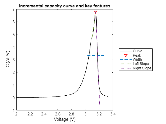
The evolution of the IC curves over the battery lifetime associates with the capacity loss of the LIB. In order to gain valuable insights from the curves, it is critical to identify the key features associated with battery degradation. One method to accomplish this is to plot incremental capacity curves across cycles.
cycleList = sort(unique(differentialTable.(bParser.CycleIndexVariable)));
cyclingPhase = "Discharge";
stepIndex = 10;
plotInterval = 30;
hPlotCurvesforCycles(differentialTable, bParser, cycleList, cyclingPhase, stepIndex, plotInterval, curveType)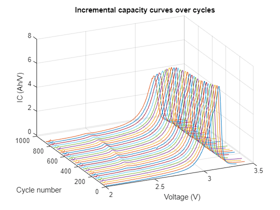
This plot illuminates the degradation patterns of LIBs, allowing for a clearer understanding of how certain features evolve as the battery ages.
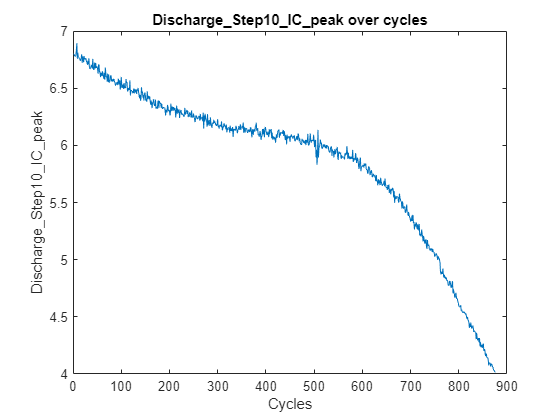
A notable observation is the decrease of peak height and peak area of the IC curve over time, which is a key indicator of battery degradation. Another significant observation is the shift of DV curve peak location across cycles, which provides insights of the changing health status.
Based on the observations, you can identify the features that are more relevant to battery degradation, such as peak height, peak location, and peak area, which decrease as the cycle number increases.
featureName = "Discharge_Step10_IC_peak";
hPlotFeatureOverCycles(featureTable,featureName, bParser.CycleIndexVariable);
3. Analyze general features
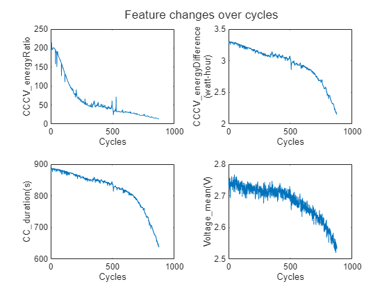
With the increase in internal resistance and loss of capacity caused by repeated charging and discharging, the time for a battery to reach terminal voltage during charging and discharging can be gradually shortened. Measurements also fluctuate over time. Therefore, in addition to curve-related features, you can extract a wide array of other features, including statistical metrics, domain-specific characteristics, and features specific to different cycling modes.
Visualizing these features over time helps to understand the feature trajectory. Features such as Discharge_Step10_CCCV_energyRatio, Discharge_Step10_CCCV_energyDifference, Discharge_Step10_CC_duration, Discharge_Voltage_mean, show significant changes of the trend over cycles. As expected, the duration of the CC mode decreases as battery capacity degrades, since the battery reaches terminal voltage earlier. This early termination of the CC mode also results in a lower average voltage and decreased CC energy. Consequently, the energy difference and ratio between CC and CV modes degrade over time.
featureNameList = ["Discharge_Step10_CCCV_energyRatio", "Discharge_Step10_CCCV_energyDifference", "Discharge_Step10_CC_duration", "Discharge_Voltage_mean"];
hPlotFeaturesTiles(featureTable, featureNameList, bParser.CycleIndexVariable)
Conclusion
This example provides a comprehensive guide on using batteryTestDataParser and batteryTestFeatureExtractor for effective data preparation, data analysis and feature extraction from battery data. The workflow includes:
Ingesting raw data from battery cyclers and converting it into a standardized format for analysis;
Identifying data anomalies that may affect analysis accuracy;
Evaluating the data and features through extensive visualization;
Gaining deeper insights into battery performance through the analysis of differential curves and extracted features.
The next step involves employing feature selection algorithms to automate the identification of relevant features. These selected features can then be utilized to train machine learning or deep learning models for various applications within the battery predictive maintenance domain.
References
[1] Severson, K.A., Attia, P.M., Jin, N. et al*.* "Data-driven prediction of battery cycle life before capacity degradation." Nat Energy 4, 383–391 (2019). https://doi.org/10.1038/s41560-019-0356-8
See Also
batteryTestFeatureExtractor | batteryTestDataParser | extract | computeDifferentialCurves | segmentData