Estimate Battery State of Health from EIS Measurements

Dataset

This example uses the KIT NMC Battery Aging Dataset [1]. It contains EIS measurements from 131 commercial nickel-rich (NMC) lithium-ion cells aged under various conditions (different charge/discharge rates, temperatures, and depth-of-discharge windows) for over one year. The diversity of aging conditions ensures the model learns general degradation patterns rather than condition-specific trends.

The data is preprocessed to include only valid measurements at 50% SOC, room temperature (25°C), and charging direction. This standardized measurement condition ensures consistent comparison across check-ups and cells — impedance varies significantly with SOC and temperature, so controlling these factors isolates the aging signal.

Load and Explore Data

Load the preprocessed EIS dataset. The table contains 131 cells and 1330 EIS sweeps with SOH ranging from 37.7% to 100.0%. Each row represents one EIS sweep with the following columns:

url = 'https://ssd.mathworks.com/supportfiles/predmaint/batteryagingdata/KIT/EISDataSingleOC.zip';
downloadFolder = fullfile(tempdir,tempname);
loc = websave('WindTurbine_FarmA', url);
unzip(loc, pwd)
load("eisCyclesData.mat", "eisData")
head(eisData, 5)

    cellIndex     soh            f              z_re             z_im     
    _________    ______    _____________    _____________    _____________

        1           100    {28×1 double}    {28×1 double}    {28×1 double}
        1        99.974    {28×1 double}    {28×1 double}    {28×1 double}
        2           100    {28×1 double}    {28×1 double}    {28×1 double}
        2        99.866    {28×1 double}    {28×1 double}    {28×1 double}
        2        99.967    {28×1 double}    {28×1 double}    {28×1 double}

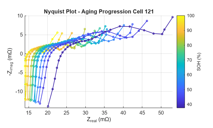
Visualize how EIS spectra change with aging for a single cell (cell 121) that has a wide SOH range. The Nyquist plot shows impedance spectra trends at different aging stages, colored by SOH:

These systematic shape changes in the Nyquist plot motivate extracting geometric features (intercepts, arc dimensions, and tail slope) as quantitative health indicators for SOH estimation.

oneCellSweeps = eisData(eisData.cellIndex == 121, :);
sweepIndices = round(linspace(1, height(oneCellSweeps), 12));
colors = flipud(parula(numel(sweepIndices)));
figure
hold on
for k = 1:numel(sweepIndices)
    s = sweepIndices(k);
    Zr = oneCellSweeps.z_re{s};
    Zi = oneCellSweeps.z_im{s};
    plot(Zr, Zi, "-o", Color=colors(k,:), MarkerSize=3, LineWidth=1.2)
end
hold off
xlabel("Z_{real} (m\Omega)")
ylabel("-Z_{imag} (m\Omega)")
title("Nyquist Plot - Aging Progression Cell 121")
axis equal
grid on
cb = colorbar;
clim([min(oneCellSweeps.soh), max(oneCellSweeps.soh)])
ylabel(cb, "SOH (%)")

Extract and Select EIS Features

Extract EIS features using batteryEISFeatures to quantify the Nyquist plot shape changes. The function identifies R0, arc features and tail features from each spectrum. These geometric features capture the physical degradation mechanisms that affect battery impedance. Call the function on the first sweep with plotting enabled to visualize which geometric features are extracted from the Nyquist plot. The first few high-frequency points are excluded here because they fall in the inductive region (negative imaginary impedance) and are not relevant to the capacitive arc and tail features.

allFeatures = batteryEISFeatures(eisData.z_re{1}(6:end), eisData.z_im{1}(6:end), eisData.f{1}(6:end), Plot=true);

Loop over the remaining sweeps to build a complete feature table with one row per EIS sweep and one column per feature. Each value is a scalar measurement extracted from the impedance spectrum geometry. This compact representation reduces a full frequency-domain spectrum into a small set of interpretable health indicators. The first sweep was already processed above to initialize the table structure.

for s = 2:height(eisData)
    allFeatures(s,:) = batteryEISFeatures(eisData.z_re{s}, eisData.z_im{s}, eisData.f{s});
end
head(allFeatures, 5)

      R0      R0_Frequency    TailSlope    TailIntercept_Zreal    Arc1_End_Zreal    Arc1_End_Zimg    Arc1_Width    Arc1_Peak_Zreal    Arc1_Peak_Zimg    Arc1_Peak_Frequency    Arc1_End_Frequency
    ______    ____________    _________    ___________________    ______________    _____________    __________    _______________    ______________    ___________________    __________________

    14.976       884.15        1.6334            18.341               18.241            0.366          3.2646          16.657             1.226               147.06                 6.7568      
    14.988       851.79         1.373             18.08               18.269             0.46          3.2814          16.245              1.15                  100                  3.125      
    14.374       899.11        1.3936            18.392                18.46            0.323          4.0865          16.382             1.201               147.06                 6.7568      
    14.383       792.57        1.2695            18.189                18.52            0.309          4.1374          16.198             1.227               147.06                      5      
    14.432       786.81        1.3322            18.227               18.467            0.444          4.0355          16.944              1.12               67.568                      5      

Explore Feature Correlation with SOH

Examine which of these features correlate most strongly with SOH to identify the best predictors for the regression model. Compute the Pearson correlation coefficient between each EIS feature and SOH across all cells and sweeps. The Pearson coefficient measures the strength and direction of the linear relationship between a feature and SOH.

featureNames = allFeatures.Properties.VariableNames;
numFeatures = numel(featureNames);
allSOH = eisData.soh;
allCellIdx = eisData.cellIndex;
corrValues = zeros(numFeatures, 1);
for i = 1:numFeatures
    corrValues(i) = corr(allFeatures.(featureNames{i}), allSOH, 'Rows', 'complete');
end

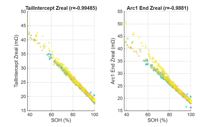
Visualize the top two most correlated features as scatter plots. Each point represents one EIS sweep, colored by cell index to verify that the trend holds across different cells (not just within a single cell). Strong monotonic trends that are consistent across cells indicate features that generalize well as SOH predictors.

[~, sortIdx] = sort(abs(corrValues), "descend");
tiledlayout(1, 2)
for p = 1:2
    nexttile
    fi = sortIdx(p);
    vals = allFeatures.(featureNames{fi});
    scatter(allSOH, vals, 15, allCellIdx, "filled", MarkerFaceAlpha=0.5)
    xlabel("SOH (%)")
    fLabel = strrep(featureNames{fi}, "_", " ");
    if contains(featureNames{fi}, ["R0" "Zreal" "Zimg" "Width" "Intercept"])
        fLabel = fLabel + " (m\Omega)";
    end
    ylabel(fLabel)
    title(strrep(featureNames{fi}, "_", " ") + " (r=" + corrValues(fi) + ")")
    grid on
end

Select Key Features

Select a compact subset of features that are most predictive of SOH, discarding noisy or redundant inputs that could lead to overfitting. Rank all features by their absolute Pearson correlation with SOH and apply a threshold of 0.8. The bar chart below visualizes this selection — features are sorted in descending order of |r|, and the red dashed line marks the cutoff.

figure
bar(abs(corrValues(sortIdx)))
hold on
yline(0.8, "r--", "Threshold", LineWidth=1.5)
hold off
xticks(1:numFeatures)
xticklabels(strrep(featureNames(sortIdx), "_", " "))
xtickangle(45)
ylabel("|Correlation with SOH|")
title("Feature Correlation with SOH")
grid on

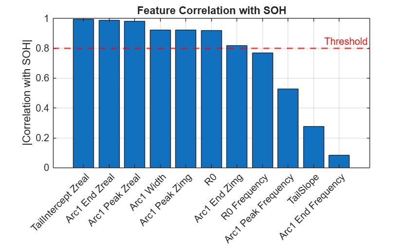
Features above the threshold are retained as model inputs. This reduces the feature space to a compact, interpretable subset that captures the dominant impedance changes associated with aging. Fewer input features also improve training efficiency and reduce the risk of multicollinearity. With informative features identified, the next step is to split the data and build a predictive model that maps these EIS features to SOH.

topFeatureIdx = find(abs(corrValues) >= 0.8);
topFeatureNames = featureNames(topFeatureIdx);

Build SOH Prediction Model

Split data into training and test sets at the cell level using an 80/20 hold-out partition. Cell-level splitting ensures all sweeps from a given cell appear in only one set. This is important because consecutive EIS measurements from the same cell are highly correlated — if some sweeps from a cell appear in training and others in testing, the model can exploit this correlation rather than learning generalizable degradation patterns. By splitting at the cell level, the test set evaluates how well the model predicts SOH for entirely unseen cells, which better reflects real-world deployment where the model encounters new batteries.

rng(0, "twister");
uniqueCells = unique(allCellIdx);
cv = cvpartition(numel(uniqueCells), "HoldOut", 0.2);
trainCells = uniqueCells(training(cv));
testCells = uniqueCells(test(cv));

trainIdx = ismember(allCellIdx, trainCells);
testIdx = ismember(allCellIdx, testCells);

xTrain = allFeatures{trainIdx, topFeatureNames};
yTrain = allSOH(trainIdx);
xTest = allFeatures{testIdx, topFeatureNames};
yTest = allSOH(testIdx);

Train Model

Train a Gaussian process regression (GPR) model to map the selected EIS features to SOH. GPR is a non-parametric Bayesian method that models the relationship between inputs and outputs as a distribution over functions. It is well-suited for this problem because it captures nonlinear relationships without requiring manual specification of the model form.

The squared exponential kernel assumes smooth, continuous degradation trends, which aligns with the gradual nature of battery aging. Input standardization ensures features with different scales contribute equally.

gprModel = fitrgp(xTrain, yTrain, ...
    KernelFunction="squaredexponential", ...
    Standardize=true);

Evaluate Model

Predict SOH on the held-out test cells. The GPR model returns both a point estimate and a prediction standard deviation for each sample. The standard deviation quantifies how confident the model is — larger values indicate the test point lies far from the training data in feature space.

Compute performance metrics to assess prediction quality:

[yPred, yStd] = predict(gprModel, xTest);
rmseVal = sqrt(mean((yTest - yPred).^2));
ssRes = sum((yTest - yPred).^2);
ssTot = sum((yTest - mean(yTest)).^2);
r2Val = 1 - ssRes/ssTot;

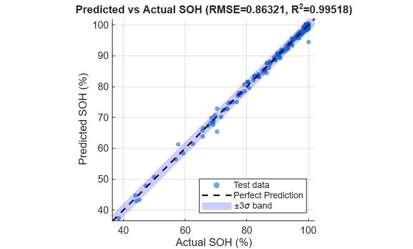
Visualize prediction accuracy with a predicted-vs-actual scatter plot. The black dashed line is the ideal reference — points on this line represent perfect predictions. The shaded blue band shows ±3σ of the average prediction uncertainty, giving a visual sense of the model's confidence envelope. Points scattered tightly around the diagonal with a narrow band indicate a well-calibrated, accurate model.

figure
hold on
scatter(yTest, yPred, 20, "filled", MarkerFaceAlpha=0.6)
sohLim = [min(yTest)-2, max(yTest)+2];
plot(sohLim, sohLim, "k--", LineWidth=1.5)
xRange = linspace(sohLim(1), sohLim(2), 100);
fill([xRange, fliplr(xRange)], ...
    [xRange+3*mean(yStd), fliplr(xRange-3*mean(yStd))], ...
    "b", FaceAlpha=0.2, EdgeColor="none")
hold off
xlabel("Actual SOH (%)")
ylabel("Predicted SOH (%)")
title("Predicted vs Actual SOH (RMSE=" + rmseVal + ", R^2=" + r2Val + ")")
legend("Test data", "Perfect Prediction", "\pm3\sigma band", Location="southeast")
grid on
xlim(sohLim)
ylim(sohLim)
axis square

References

[1] Luh, M., Blank, T. et al. "Comprehensive battery aging dataset: capacity and impedance fade measurements of a lithium-ion NMC/C-SiO cell." Scientific Data 11, 1285 (2024). https://doi.org/10.1038/s41597-024-03831-x