Nonlinear State Estimation of a Degrading Battery System
This example shows how to estimate the states of a nonlinear system using an unscented Kalman filter in Simulink®. The example also illustrates how to develop an event-based Kalman filter to update system parameters for more accurate state estimation. The example runs with either Control System Toolbox™ or System Identification Toolbox™. The example does not require Predictive Maintenance Toolbox™.
Overview
Consider a battery model with the following equivalent circuit [1]
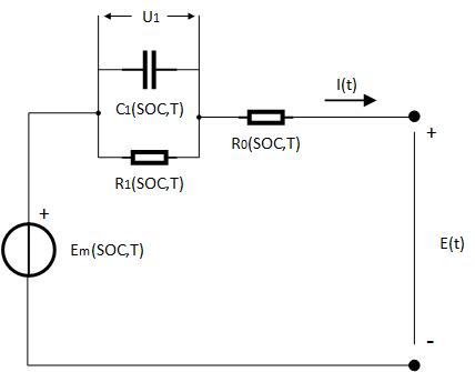
The model consists of a voltage source  , a series resistor
  and a single RC block
  and
and  . The battery alternates between charging and discharging cycles. In this example, you estimate the state of charge (SOC) of a battery model using measured currents, voltages and temperatures of the battery. You assume the battery is a nonlinear system, estimate the SOC using an unscented Kalman filter. The capacity of the battery degrades with every discharge-charge cycle, giving an inaccurate SOC estimation. Use an event-based linear Kalman filter to estimate the battery capacity when the battery transitions between charging and discharging. The estimated capacity in turn can be used to indicate the health condition of the battery.
The Simulink model contains three major components: a battery model, an unscented Kalman filter block and an event-based Kalman filter block. Further explanations are given in the following sections.
open_system('BatteryExampleUKF/')
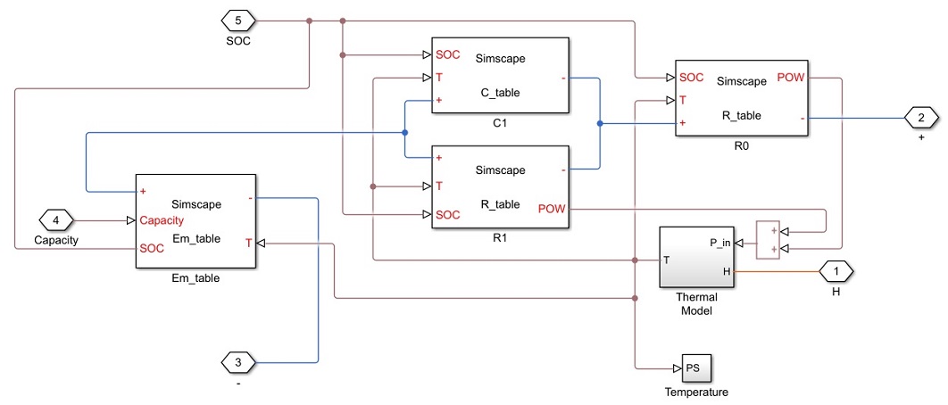
Battery Model
The battery model with thermal effects is implemented using the Simscape™ language.
The state transition equations for the battery model are given by:

where  and
and  are the thermal and SOC dependent resistor and capacitor in the RC block,
  is the voltage across capacitor ,
  is the input current,
  is the battery temperature,
  is the battery capacity (unit: Ah), and
  is the process noise.
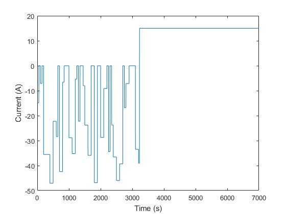
The input currents are randomly generated pulses when the battery is discharging and constant when the battery is charging, as shown in the following figure.
The measurement equation is given by:

where  is the measured voltage output,
  is the serial resistor,
 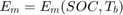 is the electromotive force from voltage source, and
  is the measurement noise.
In the model,  and are 2D look-up tables that are dependent on SOC and battery temperature. The parameters in the look-up tables are identified using experimental data [1].
Estimating State of Charge (SOC)
To use the unscented Kalman filter block, either MATLAB® or Simulink functions for the state and measurement equations need to be defined. This example demonstrates the use of Simulink functions. Since unscented Kalman filters are discrete-time filters, first discretize the state equations. In this example, Euler discretization is employed. Let the sampling time be  . For a general nonlinear system
  , the system can be discretized as
The state vectors of the nonlinear battery system are
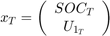 .
.
Applying Euler discretization gives the following equations:

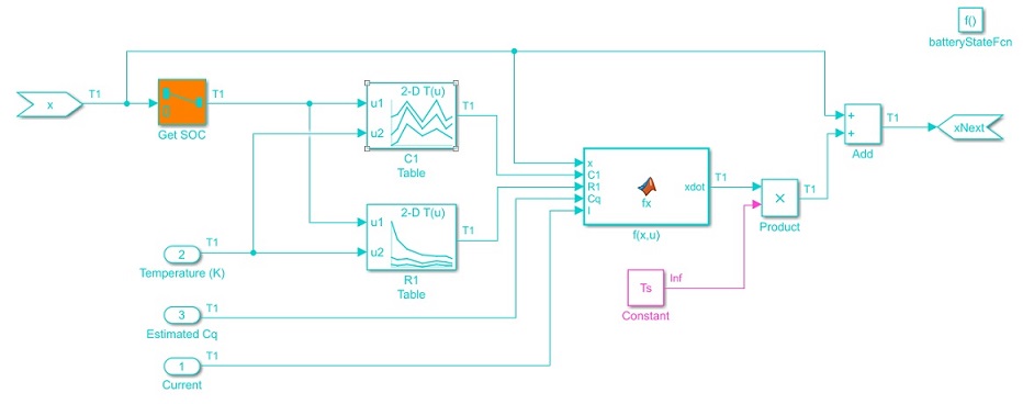
The discretized state transition equation is implemented as a Simulink function named "batteryStateFcn" shown below. The function input x is the state vector while the function output xNext is the state vector at next step, calculated using discretized state transition equations. You need to specify the signal dimensions and data type of x and xNext. In this example, the signal dimension for x and xNext is 2 and the data type is double. Additional inputs are the temperature, estimated capacity, and current. Note that the additional inputs are inputs to the state transition equations and not required by the UKF block.
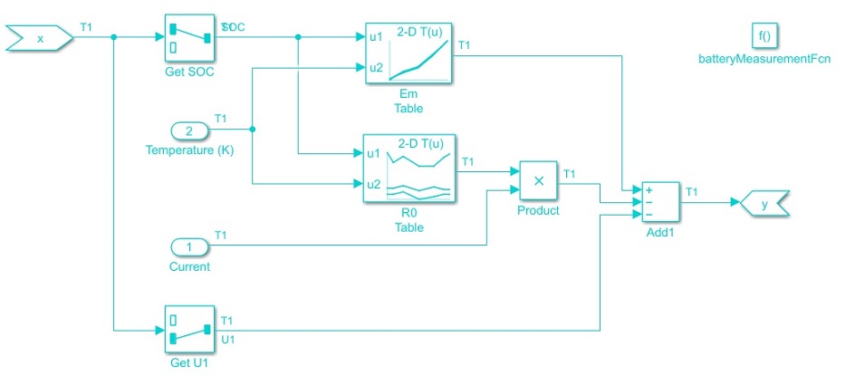
The measurement function is also implemented as a Simulink function named "batteryMeasurementFcn" as shown below.
Configure the block parameters as follows:
In the System Model tab, specify the block parameters as shown:
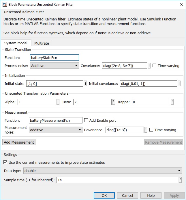
You specify the following parameters:
Function in State Transition:
batteryStateFcn.
The name of the Simulink function defined previously that implements the discretized state transition equation.
Process noise:
Additive, with time-varying covariance![$\left[ \begin{array}{cc} 2e-8 & 0 \\ 0 & 3e-7 \end{array} \right]$](../../examples/predmaint/win64/NonlinearStateEstimationOfABatterySystemExample_eq13447715808488835843.png) . The
. The Additivemeans the noise term is added to the final signals directly.
The process noise for SOC and  are estimated based on the dynamic characteristics of the battery system. The battery has nominal capacity of 30 Ah and undergoes discharge/charge cycles at an average current amplitude of 15A. Therefore, one discharging or charging process would take around 2 hours (7200 seconds). The maximum change is 100% for SOC and around 4 volts for .
The maximum changes per step in SOC and are  and
and 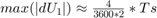 , where
  is the sampling time of the filter. In this example, is set to be 1 second.
The process noise is:
![$ W = \left[ \begin{array}{cc} (max(|dSOC|))^2 & 0 \\ 0 & (max(|dU_1|))^2 \end{array} \right] \approx \left[ \begin{array}{cc} 2e-8 & 0 \\ 0 & 3e-7 \end{array} \right] $](../../examples/predmaint/win64/NonlinearStateEstimationOfABatterySystemExample_eq09064165382790124354.png) .
.
Initial State:
 .
.
The initial value for SOC is assumed to be 100% (fully charged battery) while initial value for is set to be 0, as we do not have any prior information of .
Initial Covariance:
Initial covariance indicates how accurate and reliable the initial guesses are. Assume the maximum initial guess error is 10% for SOC and 1V for . The initial covariance matrix is set to be ![$ \left[ \begin{array}{cc} 0.01 & 0 \\ 0 & 1 \end{array} \right] $](../../examples/predmaint/win64/NonlinearStateEstimationOfABatterySystemExample_eq00624807450018571446.png) .
.
Unscented Transformation Parameters: The setting is based on [2]
     - Alpha: 1. Determine the spread of sigma points around x. Set Alpha to be 1 for larger spread.
     - Beta: 2. Used to incorporate prior knowledge of the distribution. The nominal value for Beta is 2.
     - Kappa: 0. Secondary scaling parameter. The nominal value for Kappa is 0.
Function in Measurement:
batteryMeasurementFcn.
The name of the Simulink function defined previously that implements the measurement function.
Measurement noise:
Additive, with time-invariant covariance 1e-3.
The measurement noise is estimated based on measurement equipment accuracy. A voltage meter for battery voltage measurement has approximately 1% accuracy. The battery voltage is around 4V. Equivalently, we have  . Therefore, set
  .
.
Sample Time:
 .
.
Estimating Battery Degradation
The battery degradation is modeled by decreasing capacity . In this example, the battery capacity is set to decrease 1 Ah per discharge-charge cycle to illustrate the effect of degradation. Since the degradation rate of capacity is not known in advance, set the state equation of  to be a random walk:
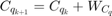
where  is the number of discharge-charge cycles and
  is the process noise.
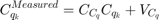
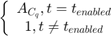
The battery is configured to automatically charge when the battery state of charge is at 30% and switch to discharging when state of charge is at 90%. Use this information to measure the battery capacity by integrating the current over a charge or discharge cycle (coulomb counting).
The measurement equation for is:
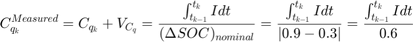
where  is the measurement noise.
The state and measurement equation of battery degradation can be put into the following state space form:
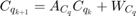
where  and
and  are equal to 1.
For the above linear system, use a Kalman filter to estimate battery capacity. The estimated from the linear Kalman filter is used to improve SOC estimation. In the example, an event-based linear Kalman filter is used to estimate . Since is measured once over a charge or discharge cycle, the linear Kalman filter is enabled only when charging or discharging ends.
Configure the block parameters and options as follows:
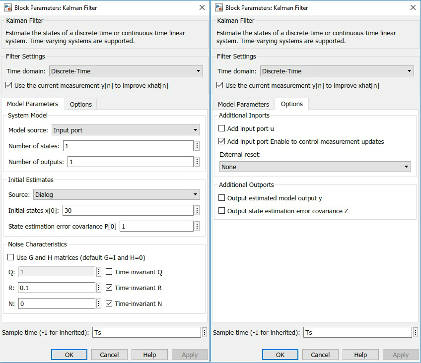
Click Model Parameters to specify the plant model and noise characteristics:
Model source:
Input Port.
To implement an event-based Kalman filter, the state equation is enabled only when the event happens. In other word, the state equation is event-based as well. For a linear system  , set the state equation to be
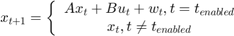 .
.
A:
 . In this example,
  . As a result,
  equals 1 all the time.
C: 1, from
 .
.
Initial Estimate Source:
Dialog. You specify initial states inInitial state x[0]
Initial states x[0]: 30. It is the nominal capacity of battery (30Ah).
Q:

This is the covariance of the process noise . Since degradation rate in the capacity is around 1 Ah per discharge-charge cycle, set the process noise to be 1.
R: 0.1. This is the covariance of the measurement noise
. Assume the capacity measurement error is less than 1%. With battery capacity of 30 Ah, the measurement noise  .
.
Sample Time: Ts.
Click Options to add input port Enable to control measurement updates. The enable port is used to update the battery capacity estimate on charge/discharge events as opposed to continually updating.
Note that setting Enable to 0 does not disable predictions using state equations. It is the reason why the state equation is configured to be event-based as well. By setting an event-based A and Q for the Kalman filter block, predictions using state equations are disabled when Enable is set to be 0.
Results
To simulate the system, load the battery parameters. The file contains the battery parameters including  ,
,  ,
,  and etc.
load BatteryParameters.mat
Simulate the system.
sim('BatteryExampleUKF')
At every time step, the unscented Kalman filter provides an estimation for SOC based on voltage measurements . Plot the real SOC, the estimated SOC, and the difference between them.
% Synchronize two time series
[RealSOC, EstimatedSOC] = synchronize(RealSOC, EstimatedSOC, 'intersection');

figure;
subplot(2,1,1)
plot(100*RealSOC,'b','LineWidth',1.5);
hold on
plot(100*EstimatedSOC,'r--','LineWidth',1);
title('State of Charge');
xlabel('Time (s)');
ylabel('SOC (%)');
legend('Actual','UKF estimate','Location','Best','Orientation','horizontal');
axis tight

subplot(2,1,2)
DiffSOC = 100*(RealSOC - EstimatedSOC);
plot(DiffSOC.Time, DiffSOC.Data, 'LineWidth', 1.5);
xlabel('Time(s)');
ylabel('\Delta SOC (%)','Interpreter','Tex');
legend('Difference between Real SOC and Estimated SOC','Location','Best')
axis tight
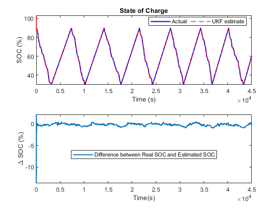
After an initial estimation error, the SOC converges quickly to the real SOC. The final estimation error is within 0.5% error. The unscented Kalman filter gives an accurate estimation of SOC.
At every discharge-charge transitions, the battery capacity is estimated to improve the SOC estimation. The battery system outputs indicator signals to inform what process the battery is in. Discharging process is represented by -1 in the indicator signals while charging process is represented by 1. In this example, changes in the indicator signals are used to determine when to enable or disable Kalman filter for capacity estimation. We plot the real and estimated capacity as well as the charge-discharge indicator signals.
figure;
subplot(2,1,1);
plot(RealCapacity,'b','LineWidth',1.5);
hold on
plot(EstimatedCapacity,'r--','LineWidth',1.5);
xlabel('Time (s)');
ylabel('Capacity (Ah)');
legend('Actual','KF estimate','Location','Best');

subplot(2,1,2);
plot(DischargeChargeIndicator.Time,DischargeChargeIndicator.Data,'b','LineWidth',1.5);
xlabel('Time(s)');
ylabel('Indicator Signal');
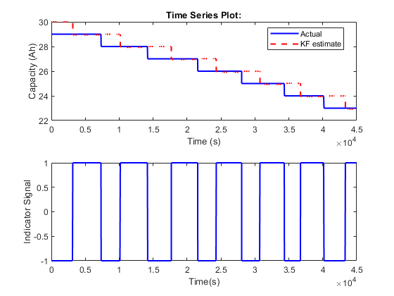
In general, the Kalman filter is able to track the real capacity. There is a half cycle delay between estimated capacity and real capacity. This delay is due to the timing of the measurements. The battery capacity degradation calculation occurs when one full discharge-charge cycle ends. The coulomb counting gives a capacity measurement based on the previous discharge or charge cycle.
Summary
This example shows how to use the Simulink unscented Kalman filter block to perform nonlinear state estimation for a lithium battery. In addition, steps to develop an event-based Kalman filter for battery capacity estimation are illustrated. The newly estimated capacity is used to improve SOC estimation in the unscented Kalman filter.
Reference
[1] Huria, Tarun, et al. "High fidelity electrical model with thermal dependence for characterization and simulation of high power lithium battery cells." Electric Vehicle Conference (IEVC), 2012 IEEE International. IEEE, 2012.
[2] Wan, Eric A., and Rudolph Van Der Merwe. "The unscented Kalman filter for nonlinear estimation." Adaptive Systems for Signal Processing, Communications, and Control Symposium 2000. AS-SPCC. IEEE, 2000.