Detect Aging Severity in Power Converters
Power converters change electrical energy from one form to another to meet the requirements of the applications they support. They are a key part of electrical devices across industries such as consumer electronics, renewable energy systems, and industrial equipment. Two of the common causes of power-converter degradation are capacitor and semiconductor degradation. This example shows how to use a power converter modeled in Simscape™ Electrical™ to simulate semiconductor-based degradation in IGBT (Insulated Gate Bipolar Transistors) switches. The example then uses this synthetic data to build a predictive maintenance algorithm that can detect age-induced degradation, or aging severity, in the power converter.
Load the Model
mdl = 'Three_Phase_Inverter.slx';
load_system(mdl);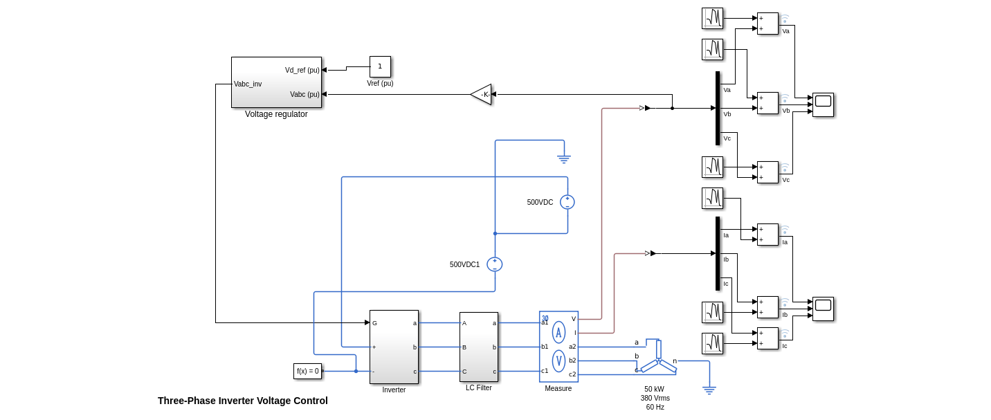
The model represents a three-phase inverter that uses an ideal voltage source. The model includes the following elements:
A three-phase inverter that consists of six IGBTs (Insulated Gate Bipolar Transistors), two for each phase
An LC filter to smooth out switching noise, and voltage fluctuations
A voltage regulator to provide a stable and consistent output voltage regardless of variations in input voltage or load conditions
Generate Data for Impacts of Aging Severity
As IGBTs age, degradation leads to changes that impact performance, reliability, and overall lifespan. Aging severity changes include the following primary characteristics:
Threshold voltage: Minimum gate-emitter voltage required to turn on the IGBT and allow a significant current to flow between the collector and emitter
Transconductance: Change in the collector current per unit change in the gate-emitter voltage, while keeping the collector-emitter voltage constant
On-state resistance: Resistance encountered by the current flowing through the IGBT when it is in the On state.
The example focuses on simulating a changing On-state resistance to model aging of the IGBT. When the device is at the end of its life, the On-state resistance decreases by about 20% to 25% compared to its nominal value [1]. Note that On-state resistance cannot be directly measured. Instead the output voltage and current are used to estimate the On-state resistance.
Vary the On-state resistance by changing the RON parameter (On resistance) of the IGBT blocks in the model to simulate aging of the power converter. Each simulation selects one of the six IGBTs at random and sets the IGBT RON value to a value indicating either a healthy or degraded state. Create Simulink.SimulationInput objects with the selected resistance value for the IGBT of choice. Add random noise to the current and voltage measurements to mimic real-world conditions. To train a machine learning model to distinguish between the different aging states, generate twenty simulations for each aging state. Define the RON values as defined in [1]. Define the location of aging and aging severity state of the selected switch for each simulation.
RON = [7e-3,6.3e-3,5.7e-3,5e-3];
AgingSeverity = ["Healthy", "Mild", "Moderate", "High"];
blockPath = "Three_Phase_Inverter/Inverter/";
locn = ["AH", "AL", "BH", "BL", "CH", "CL"];
scn = {'.. Generating Healthy data!';'.. Generating aging data for phase A';...
      '.. Generating aging data for phase B';'.. Generating aging data for phase C'; };

numSimPerSeverity = 20;
agingLocation = repmat([1,2;3,4;5,6],[1, ceil(numSimPerSeverity/2)]);
ageSeverity = repmat([2 2 3 3 4 4],[1, ceil(numSimPerSeverity/6)]);
Create Simulink.SimulationInput objects for each aging parameter choice:
simin = Simulink.SimulationInput.empty;
for iScn = 1:length(scn)
    for iSim = 1:numSimPerSeverity
        simin(end+1) = Simulink.SimulationInput(mdl);
        if iScn == 1
            selectedLocation = randsample(1:6,1);

            blockPath_ = strjoin([blockPath,locn(selectedLocation)], '');
            Ron = RON(iScn);

            fileName = ['Test_data_Healthy_file_',num2str(iSim),'.xlsx'];
            simin(end) = simin(end).setBlockParameter(blockPath_, 'Ron', num2str(Ron));
        else
            selectedLocation = agingLocation(iScn-1,iSim);
            selectedSeverity = ageSeverity(iSim);

            blockPath_ = strjoin([blockPath,locn(selectedLocation)], '');
            Ron = RON(selectedSeverity);
            simin(end) = simin(end).setBlockParameter(blockPath_, 'Ron', num2str(Ron));
        end
    end
end
Use the generateSimulationEnsemble function to run the simulations defined by the Simulink.SimulationInput objects defined above and store the results in a folder called Data.
if ~isfolder("Data")
    mkdir("Data");
end

generateSimulationEnsemble(simin, 'Data', 'ShowProgress',false);
Create a simulationEnsembleDatastore from the stored results in the Data folder. Generate the value for the condition variable called AgingSeverity for each mat file in the Data folder, using the RON parameter value.
sens = simulationEnsembleDatastore('Data');

sens.SelectedVariables = "SimulationInput";
sens.ConditionVariables = "AgingSeverity";

reset(sens);

while hasdata(sens)
    data = read(sens);
    Ron = str2double(data.SimulationInput{1}.BlockParameters.Value);
    [~, loc] = min(abs(Ron-RON));
    writeToLastMemberRead(sens,'AgingSeverity',AgingSeverity(loc));
end
Read the Generated Data into MATLAB for Feature Extraction
Read all the data into the MATLAB® workspace for feature extraction and model training. Plot the current measurement Ia from one of the Healthy and High aging severity data sets to visualize any differences between the two cases.
sens.SelectedVariables = ["Ia", "Ib", "Ic", "Va", "Vb", "Vc", "AgingSeverity"];

measuredData = readall(sens);

tiledlayout;
nexttile;
Ia_healthy = measuredData.Ia{find(measuredData.AgingSeverity == "Healthy", 1)};
plot(Ia_healthy.Time, Ia_healthy.Data, '--'); hold on;
Ia_high_severity = measuredData.Ia{find(measuredData.AgingSeverity == "High", 1)};
plot(Ia_high_severity.Time, Ia_high_severity.Data, '-.'); hold off;
legend(["Healthy", "High Severity"]);
title("Current Measurement on First Phase");
nexttile;
Vb_healthy = measuredData.Vb{find(measuredData.AgingSeverity == "Healthy", 1)};
plot(Vb_healthy.Time, Vb_healthy.Data, '--'); hold on;
Vb_high_severity = measuredData.Vb{find(measuredData.AgingSeverity == "High", 1)};
plot(Vb_high_severity.Time, Vb_high_severity.Data, '-.'); hold off;
legend(["Healthy", "High Severity"]);
title("Voltage Measurement on Second Phase");
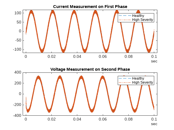
As the plots show, the current measurements for the two cases looks similar, making it very difficult to distinguish between them visually. To identify characteristics that can be used to distinguish between the various aging severity conditions, extract time-domain and frequency-domain features from the data.
Open the Diagnostic Feature Designer app with measuredData specified as the input argument. As an alternative to using the app itself, you can use app-generated MATLAB code from a previous session. Set openDFDApp to false to use the code in diagnosticFeatures_IGBT and to true to open the app.
openDFDApp = false;
if openDFDApp
    diagnosticFeatureDesigner(measuredData);
else
    FeatureTable = diagnosticFeatures_IGBT(measuredData);
end
Starting parallel pool (parpool) using the 'Processes' profile ...
Connected to parallel pool with 4 workers.
In the app, import the data and select all the imported signals for the Time Domain Signal Features computation.
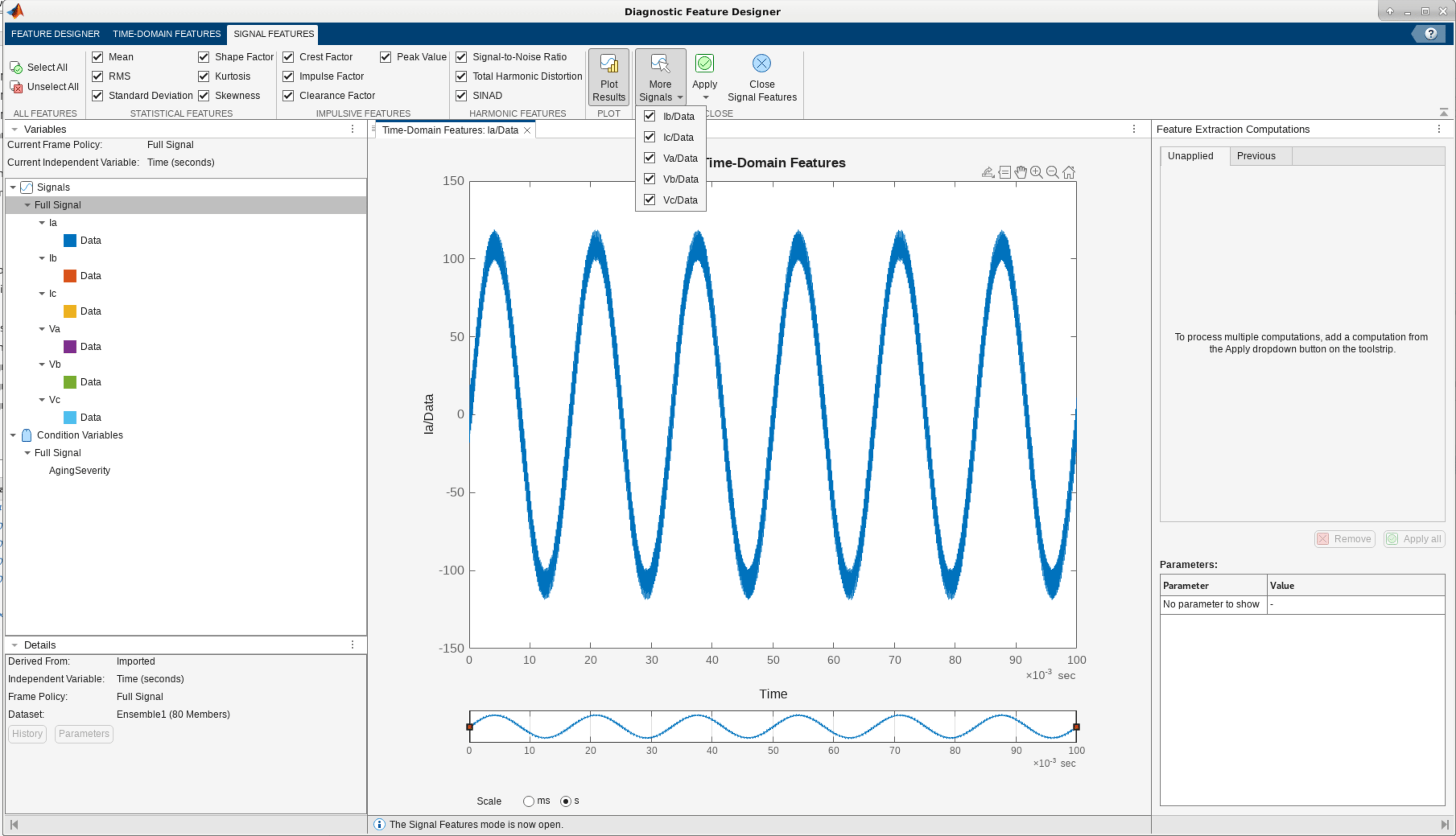
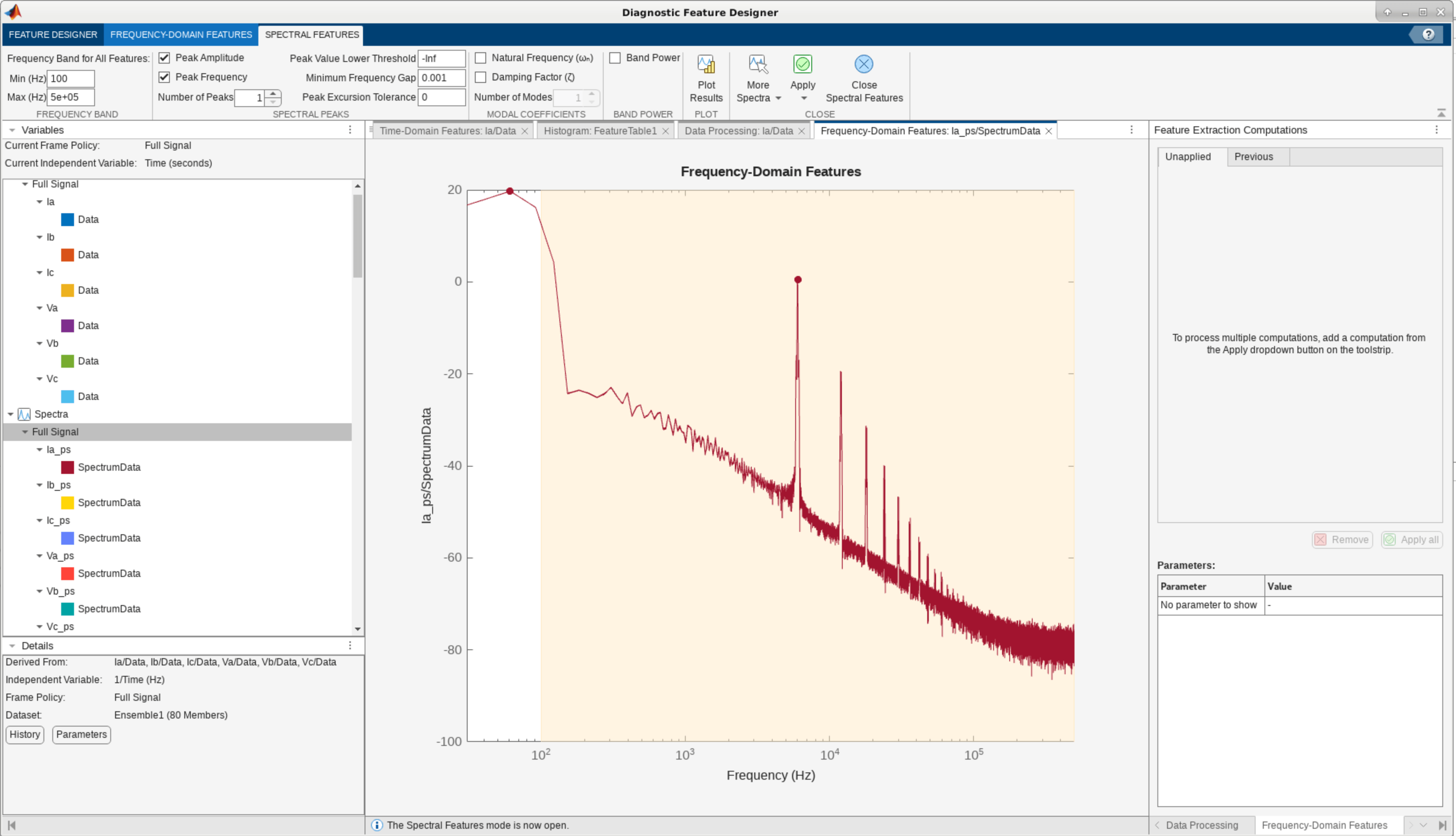
The current and voltage measurements for each of the phases are sinusoidal signals. For such signals, frequency-domain features capture key characteristics such as peak amplitudes and location, which tend to vary as the system behavior evolves. In the app, compute the power spectrum using Welch's Method for all the imported signals, and then, from these spectra, compute spectral features using the Frequency Domain features menu.
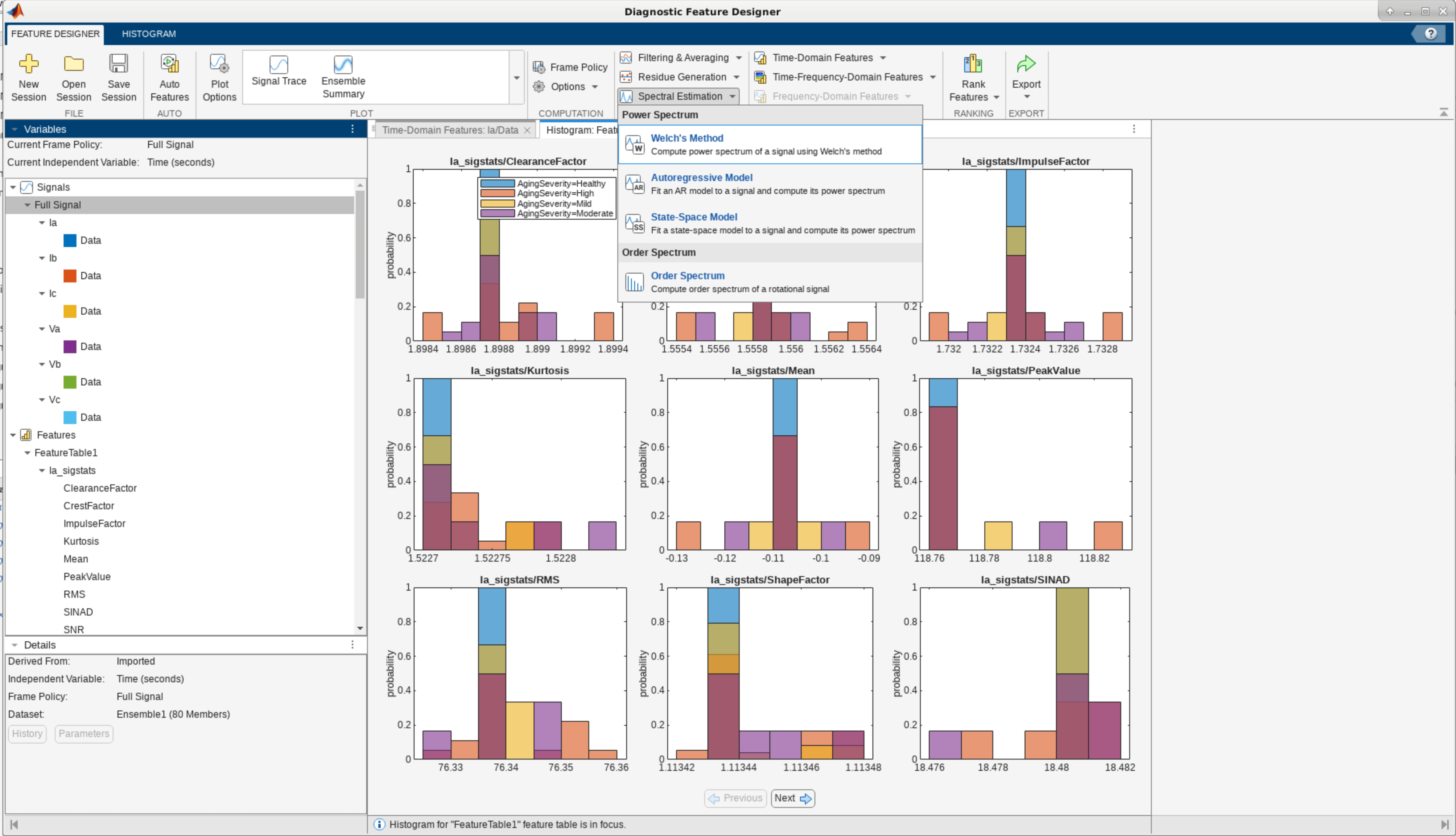
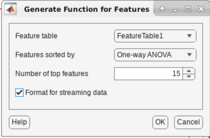
Rank the features using the default One-way Anova method and export the top fifteen features to the MATLAB workspace. Also export a MATLAB function to use later in the example for deployment. Use Generate Functions for Features and select Format for streaming data. Click OK and name the saved function as diagnosticFeatures_streaming_IGBT.m.
head(FeatureTable,5);
    AgingSeverity    Ia_sigstats/THD    Ic_sigstats/ClearanceFactor    Ic_sigstats/CrestFactor    Ic_sigstats/ImpulseFactor    Ic_sigstats/PeakValue    Ic_sigstats/THD    Va_sigstats/Kurtosis    Va_sigstats/THD    Vc_sigstats/THD    Ia_ps_spec/PeakAmp1    Ib_ps_spec/PeakAmp1    Ic_ps_spec/PeakAmp1    Va_ps_spec/PeakAmp1    Vb_ps_spec/PeakAmp1    Vc_ps_spec/PeakAmp1
    _____________    _______________    ___________________________    _______________________    _________________________    _____________________    _______________    ____________________    _______________    _______________    ___________________    ___________________    ___________________    ___________________    ___________________    ___________________

      "Healthy"          -28.468                  1.9023                       1.5578                      1.7353                      118.7                -28.677               1.5228               -28.461            -28.683              1.1063                 1.1053                 1.1137                 9.2235                 9.2155                  9.285
      "Healthy"          -28.468                  1.9023                       1.5578                      1.7353                      118.7                -28.677               1.5228               -28.461            -28.683              1.1063                 1.1053                 1.1137                 9.2235                 9.2155                  9.285
      "Healthy"          -28.468                  1.9023                       1.5578                      1.7353                      118.7                -28.677               1.5228               -28.461            -28.683              1.1063                 1.1053                 1.1137                 9.2235                 9.2155                  9.285
      "Healthy"          -28.468                  1.9023                       1.5578                      1.7353                      118.7                -28.677               1.5228               -28.461            -28.683              1.1063                 1.1053                 1.1137                 9.2235                 9.2155                  9.285
      "Healthy"          -28.468                  1.9023                       1.5578                      1.7353                      118.7                -28.677               1.5228               -28.461            -28.683              1.1063                 1.1053                 1.1137                 9.2235                 9.2155                  9.285
gplotmatrix(FeatureTable{:, 2:6}, [], FeatureTable.AgingSeverity)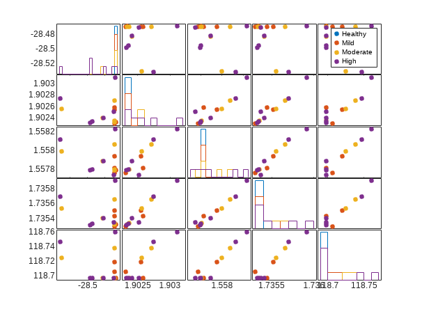
Train a Model to Detect Aging Severity
Use the cvpartition function to partition the data in FeatureTable into training and test partitions to use for training and validating a machine learning model. Set the random number generator to default to ensure repeatability of results in the example.
rng("default")

n = height(FeatureTable);
hpartition = cvpartition(n,'Holdout',0.3);
idxTrain = training(hpartition);
FeatureTable_Train = FeatureTable(idxTrain,:);
idxTest = test(hpartition);
FeatureTable_Test = FeatureTable(idxTest,:);
To find a suitable machine learning model, use fitcauto to automatically select a classification model with optimized hyperparameters. Given predictor and response data, fitcauto automatically creates a selection of classification model types with different hyperparameter values. Limit the model space to "svm" to obtain faster search and training time for this example. Also set the MaxObjectiveEvaluations to 30 to increase the number of hyperparameter options that the function searches. Set MaxTime to 60 to limit the time spent searching for the best model and hyperparameters. The software picks these values based on experimentation. The values might need to be recalculated for other data sets.
mdl = fitcauto(FeatureTable_Train, "AgingSeverity", "Learners", ["svm"],...
    "HyperparameterOptimizationOptions", struct("UseParallel",true, "Verbose", 0, "showplot", false, "MaxObjectiveEvaluations", 40, "MaxTime", 60));
Validate the trained model with test data and generate a confusion matrix to visualize the performance of the trained model for the test data set.
[eSeverity, eScores] = mdl.predict(FeatureTable_Test);

confusionchart(FeatureTable_Test.AgingSeverity, string(eSeverity))
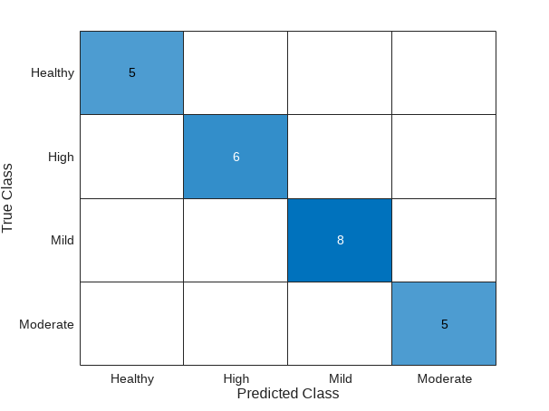
The confusion chart indicates that the selected model is able to identify the different aging severities accurately.
Generate a MEX File for Selected Model and Validate Performance
Now that you have identified a suitable model with good performance, generate code for this algorithm. This process includes generating code for feature extraction and model inference. To generate MATLAB code suitable for C/C++ code generation in the app, use the diagnosticFeatures_streaming_IGBT.m file that you generated previously.
To prepare for code generation, save the trained model using saveLearnerForCoder function:
testData = measuredData(1,:);
saveLearnerForCoder(mdl,'SVMModel');
Create a function called classifyAgeSeverity.m that accepts testData as input and returns the identified aging severity state.
type("classifyAgeSeverity.m")function label = classifyAgeSeverity(x) %#codegen
%ClassifyAgeSeverity function accepts a timetable representing the current
%batch of measurements from the power converter system. The predefined
%features are computed. and the trained model is used to detect the
%aging severity of the power converter for this batch of data.
Mdl = loadLearnerForCoder('SVMModel');
features = diagnosticFeatures_streaming_IGBT(x);
label = predict(Mdl,features);
end
Use the codegen function to generate a MEX file for the classifyAgeSeverity.m file.
codegen classifyAgeSeverity -args {testData}
Code generation successful.
Validate the generated MEX file by generating a confusion matrix for testdata in MATLAB and from the MEX file.
total_test_Samples = 5;
random_Index = randsample(height(measuredData), total_test_Samples);
for rI = 1:total_test_Samples
    testData = measuredData(random_Index(rI), :);
    mlResponse{rI} = classifyAgeSeverity(testData); %#ok<*SAGROW>
    MEXResponse{rI} = classifyAgeSeverity(testData);
end

disp('MATLAB Response\n');
MATLAB Response\n
disp([mlResponse{:}]); {'Mild'} {'Healthy'} {'High'} {'Moderate'} {'Mild'}
disp('\nMex Response\n');\nMex Response\n
disp([MEXResponse{:}]); {'Mild'} {'Healthy'} {'High'} {'Moderate'} {'Mild'}
The results of calling the MATLAB file and MEX file for the same input data are identical. The codegen function can be used for other build types such as lib, dll, or exe to suite your application needs.
References
[1] https://eprints.whiterose.ac.uk/135441/1/IECON_2018_Evan_Dimech_John_Dawson_Postprint.pdf
See Also
generateSimulationEnsemble | Diagnostic Feature
Designer | cvpartition | fitcauto | confusionchart | saveLearnerForCoder | codegen (MATLAB Coder)