RUL Estimation Using RUL Estimator Models
Predictive Maintenance Toolbox™ includes some specialized models designed for computing RUL from different types of measured system data. These models are useful when you have historical data and information such as:
Run-to-failure histories of machines similar to the one you want to diagnose
A known threshold value of some condition indicator that indicates failure
Data about how much time or how much usage it took for similar machines to reach failure (lifetime)
RUL estimation models provide methods for training the model using historical data and using it for performing prediction of the remaining useful life. The term lifetime here refers to the life of the machine defined in terms of whatever quantity you use to measure system life. Similarly time evolution can mean the evolution of a value with usage, distance traveled, number of cycles, or other quantity that describes lifetime.
The general workflow for using RUL estimation models is:
Choose the best type of RUL estimation model for the data and system knowledge you have. Create and configure the corresponding model object.
Train the estimation model using the historical data you have. To do so, use the
fitcommand.Using test data of the same type as your historical data, estimate the RUL of the test component. To do so, use the
predictRULcommand. You can also use the test data recursively to update some model types, such as degradation models, to help keep the predictions accurate. To do so, use theupdatecommand.
For a basic example illustrating these steps, see Update RUL Prediction as Data Arrives.
Choose an RUL Estimator
There are three families of RUL estimation models. Choose which family and which model to use based on the data and system information you have available, as shown in the following illustration.
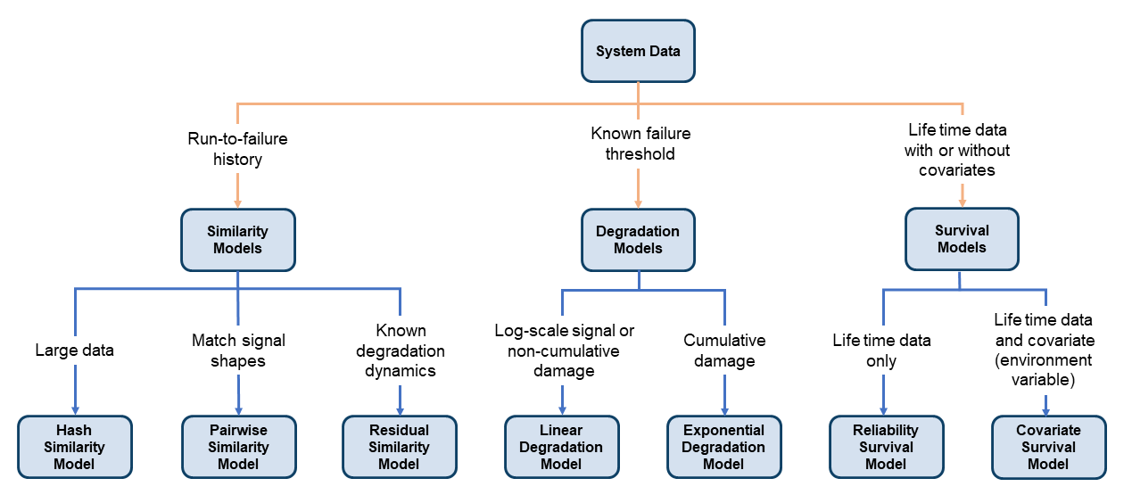
Similarity Models
Similarity models base the RUL prediction of a test machine on known behavior of similar machines from a historical database. Such models compare a trend in test data or condition-indicator values to the same information extracted from other, similar systems.
Similarity models are useful when:
You have run-to-failure data from similar systems (components). Run-to-failure data is data that starts during healthy operation and ends when the machine is in a state close to failure or maintenance.
The run-to-failure data shows similar degradation behaviors. That is, the data changes in some characteristic way as the system degrades.
Thus you can use similarity models when you can obtain degradation profiles from your data ensemble. The degradation profiles represent the evolution of one or more condition indicators for each machine in the ensemble (each component), as the machine transitions from a healthy state to a faulty state.
Predictive Maintenance Toolbox includes three types of similarity models. All three types estimate RUL by
determining the similarity between the degradation history of a test data set and the
degradation history of data sets in the ensemble. For similarity models, predictRUL
estimates the RUL of the test component as the median life span of most similar components
minus the current lifetime value of the test component. The three models differ in the ways
they define and quantify the notion of similarity.
Hashed-feature similarity model (
hashSimilarityModel) — This model transforms historical degradation data from each member of your ensemble into fixed-size, condensed, information such as the mean, total power, maximum or minimum values, or other quantities.When you call
fiton ahashSimilarityModelobject, the software computes these hashed features and stores them in the similarity model. When you callpredictRULwith data from a test component, the software computes the hashed features and compares the result to the values in the table of historical hashed features.The hashed-feature similarity model is useful when you have large amounts of degradation data, because it reduces the amount of data storage necessary for prediction. However, its accuracy depends on the accuracy of the hash function that the model uses. If you have identified good condition indicators in your data, you can use the
Methodproperty of thehashSimilarityModelobject to specify the hash function to use those features.Pairwise similarity model (
pairwiseSimilarityModel) — Pairwise similarity estimation determines RUL by finding the components whose historical degradation paths are most correlated to that of the test component. In other words, it computes the distance between different time series, where distance is defined as correlation, dynamic time warping (dtw), or a custom metric that you provide. By taking into account the degradation profile as it changes over time, pairwise similarity estimation can give better results than the hash similarity model.Residual similarity model (
residualSimilarityModel) — Residual-based estimation fits prior data to model such as an ARMA model or a model that is linear or exponential in usage time. It then computes the residuals between data predicted from the ensemble models and the data from the test component. You can view the residual similarity model as a variation on the pairwise similarity model, where the magnitudes of the residuals is the distance metric. The residual similarity approach is useful when your knowledge of the system includes a form for the degradation model.
For an example that uses a similarity model for RUL estimation, see Similarity-Based Remaining Useful Life Estimation.
Degradation Models
Degradation models extrapolate past behavior to predict the future condition. This type of RUL calculation fits a linear or exponential model to degradation profile of a condition indicator, given the degradation profiles in your ensemble. It then uses the degradation profile of the test component to statistically compute the remaining time until the indicator reaches some prescribed threshold. These models are most useful when there is a known value of your condition indicator that indicates failure. The two available degradation model types are:
Linear degradation model (
linearDegradationModel) — Describes the degradation behavior as a linear stochastic process with an offset term. Linear degradation models are useful when your system does not experience cumulative degradation.Exponential degradation model (
exponentialDegradationModel— Describes the degradation behavior as an exponential stochastic process with an offset term. Exponential degradation models are useful when the test component experiences cumulative degradation.
After you create a degradation model object, initialize the model using historical data
regarding the health of an ensemble of similar components, such as multiple machines
manufactured to the same specifications. To do so, use fit. You can
then predict the remaining useful life of similar components using predictRUL.
Degradation models only work with a single condition indicator. However, you can use principal-component analysis or other fusion techniques to generate a fused condition indicator that incorporates information from more than one condition indicator. Whether you use a single indicator or a fused indicator, look for an indicator that shows a clear increasing or decreasing trend, so that the modeling and extrapolation are reliable.
For an example that takes this approach and estimates RUL using a degradation model, see Wind Turbine High-Speed Bearing Prognosis.
Survival Models
Survival analysis is a statistical method used to model time-to-event data. It is useful when you do not have complete run-to-failure histories, but instead have:
Only data about the life span of similar components. For example, you might know how many miles each engine in your ensemble ran before needing maintenance, or how many hours of operation each machine in your ensemble ran before failure. In this case, you use
reliabilitySurvivalModel. Given the historical information on failure times of a fleet of similar components, this model estimates the probability distribution of the failure times. The distribution is used to estimate the RUL of the test component.Both life spans and some other variable data (covariates) that correlates with the RUL. Covariates, also called environmental variables or explanatory variables, comprise information such as the component provider, regimes in which the component was used, or manufacturing batch. In this case, use
covariateSurvivalModel. This model is a proportional hazard survival model which uses the life spans and covariates to compute the survival probability of a test component.
See Also
covariateSurvivalModel | reliabilitySurvivalModel | exponentialDegradationModel | linearDegradationModel | residualSimilarityModel | pairwiseSimilarityModel | hashSimilarityModel | fit | predictRUL