Train and Test Isolation Forest Time Series Anomaly Detector

This example uses:

Load the file sineWaveAnomalyData.mat, which contains two sets of synthetic 3-channel sinusoidal signals.

sineWaveNormal contains 10 sinusoids of stable frequency and amplitude. Each signal has a series of small-amplitude impact-like imperfections. The signals have different lengths and initial phases. sineWaveAbnormal contains 3 sinusoids that contain the same normal data as sineWaveNormal, but that also include anomalous data.

load sineWaveAnomalyData.mat sineWaveNormal sineWaveAbnormal

Plot input signals

Plot all 3 channels of the first three anomalous signals.

s1 = 3;
tiledlayout("vertical")
ax = zeros(s1,1);
for kj = 1:s1
    ax(kj) = nexttile;
    plot(sineWaveAbnormal{kj})
    title("Anomalous Signals")
end

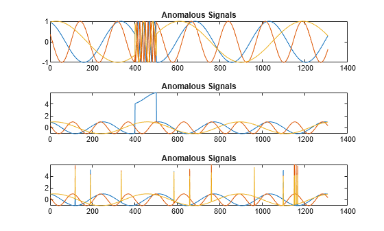
Figure contains 3 axes objects. Axes object 1 with title Anomalous Signals contains 3 objects of type line. Axes object 2 with title Anomalous Signals contains 3 objects of type line. Axes object 3 with title Anomalous Signals contains 3 objects of type line.

sineWaveAbnormal contains three signals, all of the same length. Each signal in the set has one or more anomalies.

All channels of the first signal have an abrupt change in frequency that lasts for a finite time.
The second signal has a finite-duration amplitude change in one of its channels.
The third signal has spikes at random times in all channels.

Create Detector

Use the timeseriesIforestAD detector to create an Isolated Forest detector with 3 channels and default options.

detector_tsif = timeSeriesIforestAD(3)

detector_tsif = 
  TimeSeriesIForestDetector with properties:

                  NumLearners: 100
    NumObservationsPerLearner: []
                  NumChannels: 3
                    IsTrained: 0
                 WindowLength: 10
               TrainingStride: 1
              DetectionStride: 10
                    Threshold: []
              ThresholdMethod: "kSigma"
           ThresholdParameter: 3
            ThresholdFunction: []
                Normalization: "zscore"
            FeatureExtraction: 1

Train detector using the normal data.

detector_tsif = train(detector_tsif,sineWaveNormal);

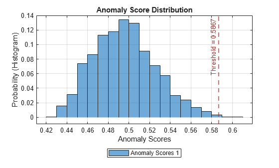
View the threshold that train computes and saves within detector_tsif. This computed value is influenced by random factors, such as which subsets of the data are used for training, and can change somewhat for different training sessions and different machines.

thresh = detector_tsif.Threshold

thresh = 
0.5867

Plot the histogram of the anomaly scores for the normal data. Each score is calculated over a single detection window. The threshold, plotted as a vertical line, does not always completely bound the scores.

plotHistogram(detector_tsif,sineWaveNormal);

Figure contains an axes object. The axes object with title Anomaly Score Distribution, xlabel Anomaly Scores, ylabel Probability (Histogram) contains 2 objects of type histogram, constantline. This object represents Anomaly Scores 1.

Use Detector to Identify Anomalies

Use the detect function to determine the anomaly scores for the anomalous data. Then, plot the anomaly scores.

results = detect(detector_tsif, sineWaveAbnormal)

results=3×1 cell array
    {130×3 table}
    {130×3 table}
    {130×3 table}

results is a cell array that contains three tables, one table for each signal. Each cell table contains three variables: WindowLabel, WindowAnomalyScore, and WindowStartIndices. Confirm the table variable names.

varnames = results{1}.Properties.VariableNames

varnames = 1×3 cell
    {'Labels'}    {'AnomalyScores'}    {'StartIndices'}

Plot Anomaly Score Distributions

Plot a histogram that shows the anomaly scores for both sets of data together, along with the threshold, for comparison.

plotHistogram(detector_tsif,sineWaveNormal,sineWaveAbnormal)

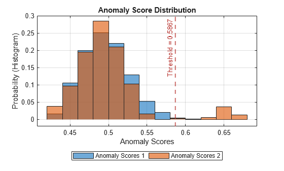
Figure contains an axes object. The axes object with title Anomaly Score Distribution, xlabel Anomaly Scores, ylabel Probability (Histogram) contains 3 objects of type histogram, constantline. These objects represent Anomaly Scores 1, Anomaly Scores 2.

The histogram uses different colors for the normal (Data 1) and anomalous (Data 2) data. Both types of data appear to the left of the threshold. To the right of threshold, Data 2 is prevalent.

Plot the detected anomalies of the third abnormal signal set.

plot(detector_tsif,sineWaveAbnormal{3})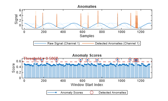

The top plot shows an overlay of red where the anomalies occur. The bottom plot shows how effective the threshold is at dividing the normal from the abnormal scores for Signal set 3.

Train and Test Isolation Forest Time Series Anomaly Detector

Plot input signals

Create Detector

Use Detector to Identify Anomalies

Plot Anomaly Score Distributions

See Also

Topics