Train and Test Time Series Statistical Process Control Anomaly Detector
Load the file sineWaveAnomalyData.mat, which contains two sets of synthetic three-channel sinusoidal signals.
sineWaveNormal contains 10 sinusoids of stable frequency and amplitude. Each signal has a series of small-amplitude impact-like imperfections. The signals have different lengths and initial phases. sineWaveAbnormal contains the same sinusoids as sineWaveNormal, but also includes anomalous data.
load sineWaveAnomalyData.mat
s1 = 3;
Plot input signals
Plot the first three anomalous input signals.
tiledlayout("vertical")
ax = zeros(s1,1);
for kj = 1:s1
    ax(kj) = nexttile;
    plot(sineWaveAbnormal{kj})
    title("Anomalous Signals")
end
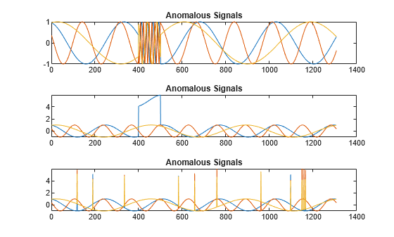
sineWaveAbnormal contains three signals, all of the same length. Each signal in the set has one or more anomalies.
All channels of the first signal have an abrupt change in frequency that lasts for a finite time.
The second signal has a finite-duration amplitude change in one of its channels.
The third signal has spikes at random times in all channels.
Create detector
Use the timeSeriesSpcAD command to create a detector with 3 channels that tracks the exponentially weighted mean average of the data.
detector_tsspc = timeSeriesSpcAD(3, Method="ewma",WindowLength=10);Train detector
Train the detector using normal data and default settings.
detector_tsspc = train(detector_tsspc,sineWaveNormal)
detector_tsspc =
  TimeSeriesSPCDetector with properties:

       NumChannels: 3
      WindowLength: 10
            Stride: 10
            Method: "ewma"
            Lambda: 0.4000
    DetectionRules: "n1"
             Level: 3
        CenterLine: [0.0056 -0.0030 -2.9131e-04]
     StandardError: [0.3533 0.3504 0.3538]
              Mean: [0.0056 -0.0030 -2.9131e-04]
             Sigma: [0.7067 0.7008 0.7075]
         MeanRange: [0.1533 0.3004 0.0925]
         IsTrained: 1
Plot detection results
Plot the detection results for sineWaveAbnormal(2)
figure(1);
detector_tsspc.plot(sineWaveAbnormal{2})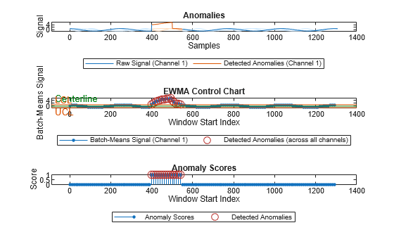
The plot shows that the detector successfully detects the anomaly.
Plot histogram
Plot the histogram of the anomaly scores.
figure(2);
detector_tsspc.plotHistogram(sineWaveNormal{2}, sineWaveAbnormal{2})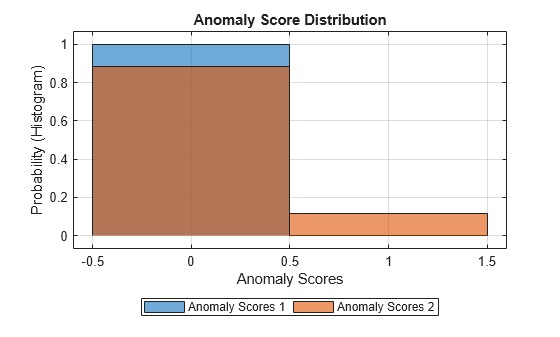
See Also
timeSeriesSpcAD | TimeSeriesSPCDetector