Cooperative Bistatic Radar I/Q Simulation and Processing
A cooperative bistatic radar is a type of bistatic radar system in which the transmitter and receiver are deliberately designed to collaborate, despite not being collocated. Unlike passive bistatic radar systems, which utilize transmissions from unrelated sources like radio and television broadcasts, cooperative bistatic radars involve transmitters that are specifically engineered to work in conjunction with one or more receivers for the purpose of detecting and tracking targets.
This example demonstrates the simulation of I/Q for a cooperative bistatic system and its subsequent signal processing for a single bistatic transmitter and receiver pair. The cooperative bistatic radar system assumes the:
Transmitter and receiver are time synchronized
Transmitter and receiver positions are known
Transmitted waveform is known
Target is a perfect electrical conductor (PEC) with no micro-motion (e.g., rotation or tumbling)
You will learn in this example how to:
Setup a bistatic scenario
Import a bistatic radar cross section (RCS) for a cone target using Antenna Toolbox™
Simulate a bistatic datacube
Perform range and Doppler processing
Form surveillance beams and null the direct path
Perform detection and parameter estimation
Format data for usage with task-oriented trackers using Sensor Fusion and Tracking Toolbox™
This example uses Radar Toolbox™, Antenna Toolbox™, and Sensor Fusion and Tracking Toolbox™.
To further explore waveform-level bistatic simulations, see the Non-Cooperative Bistatic Radar I/Q Simulation and Processing example, which shows how to simulate a passive radar with 2 signals of opportunity.
Set Up the Bistatic Scenario
First initialize the random number generation for reproducible results.
% Set random number generation for reproducibility
rng('default')
Define radar parameters for a 300 MHz cooperative bistatic radar system. The maximum range is set to 48 km, and the range resolution is 50 meters.
% Radar parameters
fc         = 3e8;                 % Operating frequency (Hz)
maxrng     = 48e3;                % Maximum range (m)
rngres     = 50;                  % Range resolution (m)
tbprod     = 20;                  % Time-bandwidth product
[lambda,c] = freq2wavelen(fc);    % Wavelength (m)
Define the pulse repetition interval (PRI) based on the maximum range using the range2time function.
% Set up scenario
pri = range2time(maxrng);
prf = 1/pri;
Create a radar scenario with the update rate set to the inverse of the PRI.
scene = radarScenario(UpdateRate=prf);
Define the platforms in the scenario. This example includes a transmitter, receiver, and a single target. The stationary transmitter and receiver are separated by 10 km. The target moves with a velocity of 150 m/s in the y-direction away from the transmitter and receiver.
% Define platforms
txPlat  = platform(scene,Position=[-5e3 0 0],Orientation=rotz(45).');
rxPlat  = platform(scene,Position=[5e3 0 0],Orientation=rotz(135).');
traj = kinematicTrajectory(Position=8e3*[cosd(60) sind(60) 0],Velocity=[0 150 0],Orientation=eye(3));
tgtPlat = platform(scene,Trajectory=traj);
Visualize the scenario using theaterPlot in the helper helperPlotScenario. The transmitter is shown below as an upward-facing blue triangle. The receiver is shown as a downward-facing blue triangle. The red, green, and blue lines form axes that indicate the orientations of the transmitter and receiver. The target is shown as a red circle with its trajectory shown as a dotted line in gray.
% Visualize the scenario
helperPlotScenario(txPlat,rxPlat,tgtPlat)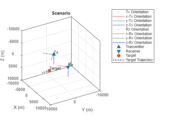
Configure Bistatic Transmitter and Receiver
Now define the bistatic transmitter.
The emitter transmits a linear frequency modulated (LFM) waveform with parameters calculated from the previously defined maximum range and range resolution.
% Waveform
bw  = rangeres2bw(rngres);
fs  = 2*bw;
waveform = phased.LinearFMWaveform(PulseWidth=tbprod/bw,PRF=1/pri,...
    SweepBandwidth=bw,SampleRate=fs);
The peak power of the transmitter is set to 500 Watts with a loss factor of 3 dB.
% Transmitter
transmitter = phased.Transmitter(PeakPower=500,Gain=0,LossFactor=3);
Define the transmit antenna as a horizontal uniform linear array (ULA) with 4 vertically oriented short dipole antenna elements spaced a half-wavelength apart. Attach the array to a phased.Radiator object.
% Transmit antenna
txAntenna   = phased.ShortDipoleAntennaElement(AxisDirection='Z');
txarray     = phased.ULA(4,lambda/2,Element=txAntenna);
radiator    = phased.Radiator(Sensor=txarray,PropagationSpeed=c);
Create a bistaticTransmitter with the previously defined waveform, transmitter, and transmit antenna.
% Bistatic transmitter
biTx        = bistaticTransmitter(Waveform=waveform, ...
    Transmitter=transmitter, ...
    TransmitAntenna=radiator);
Define the receive antenna as a horizontal uniform linear array (ULA) with 16 vertically polarized short dipole antenna elements spaced a half-wavelength apart. Attach the array to a phased.Collector object.
% Receive antenna
numPulses = 65; % Number of pulses to record
rxAntenna = phased.ShortDipoleAntennaElement(AxisDirection='Z');
rxarray   = phased.ULA(16,lambda/2,Element=rxAntenna);
collector = phased.Collector(Sensor=rxarray,...
    PropagationSpeed=c,...
    OperatingFrequency=fc);
Set the noise figure of the receiver to 6 dB.
% Receiver
receiver  = phased.Receiver(Gain=0,SampleRate=fs,NoiseFigure=6,SeedSource='Property');
Create a bistaticReceiver with the previously defined receive antenna and receiver. Set the window duration to receive 65 PRIs.
% Bistatic receiver
biRx        = bistaticReceiver(ReceiveAntenna=collector, ...
    Receiver=receiver, ...
    SampleRate=fs, ...
    WindowDuration=pri*numPulses);
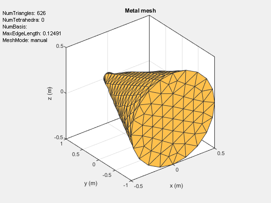
Define the Cone Target
Import the target stl file. This stl file contains a cone target with a radius of 0.05 m at one end and 0.5 meters at the other end. The height of the cone is 2 meters.
% Load cone target
p = platform;
p.FileName = 'tgtCone.stl';
p.Units = 'm';
pause(0.25)
figure
show(p)
Visualize the target in the scenario.
% Visualize cone target in theater plot
hTgtConeAxes = gca;
helperPlotTarget(hTgtConeAxes,tgtPlat)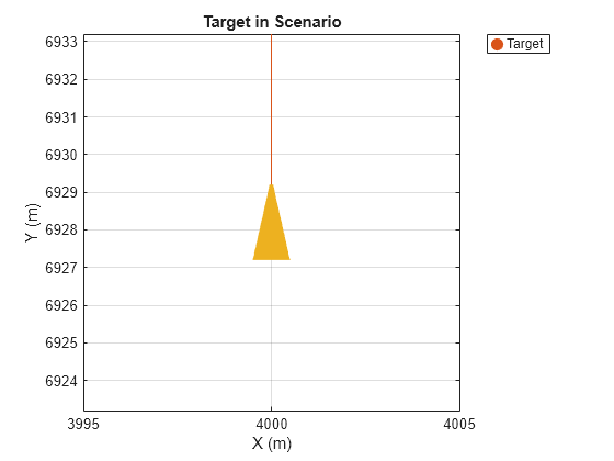
Background on Bistatic Propagation Paths
The propagation paths in this example will be modeled using free space paths.
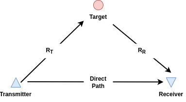
There are 3 paths modeled in this example:
Transmitter-to-receiver: This is also referred to as the direct path or baseline .
Transmitter-to-target: This is the first leg of the bistatic path and is denoted as in the diagram above.
Target-to-receiver: This is the second leg of the bistatic path and is denoted as in the diagram above.
The bistatic range is relative to the direct path and is given by
.
Simulate I/Q Data
First initialize the datacube.
% Initialize datacube
numSamples  = round(fs*pri); % Number of range samples
numElements = collector.Sensor.NumElements; % Number of elements in receive array
y           = zeros(numSamples*numPulses,numElements,like=1i); % Datacube
endIdx      = 0; % Index into datacube
Advance the scenario and get the initial time.
advance(scene);
t = scene.SimulationTime;
Use the nextTime method of the bistaticReceiver to determine the end time of the first bistatic receive window.
tEnd = nextTime(biRx);
Now receive the pulses within the bistatic receive window.
% Simulate CPI
while t < tEnd
Note that the platform poses from the platformPoses method include 3 fields needed by the bistaticFreeSpacePath function:
Position: Position of target in scenario coordinates, specified as a 1-by-3 row vector in meters.
Velocity: Velocity of platform in scenario coordinates, specified as a 1-by-3 row vector in m/s.
Orientation: Orientation of the platform with respect to the local scenario navigation frame, specified as a scalar quaternion or a 3-by-3 rotation matrix in degrees. Request a rotation matrix using the
'rotmat'flag.
The platform poses do not include target RCS. An appropriate RCS will be added after the creation of the bistatic propagation paths.
    % Get platform positions
    poses = platformPoses(scene,'rotmat');
The bistaticFreeSpacePath function creates the bistatic propagation paths.
    % Calculate paths
    proppaths = bistaticFreeSpacePath(fc, ...
        poses(1),poses(2),poses(3));
Update the bistatic propagation path ReflectionCoefficient of the target to leverage the bistatic RCS calculation from the rcs method.
    % Update target reflection coefficient
    tgtPose = poses(3);
    [Rtx,fwang] = rangeangle(poses(1).Position(:),tgtPose.Position(:),tgtPose.Orientation.');
    [Rrx,bckang] = rangeangle(poses(2).Position(:),tgtPose.Position(:),tgtPose.Orientation.');
    rcsLinear = rcs(p,fc,TransmitAngle=fwang,ReceiveAngle=bckang,Polarization="VV",Scale="linear");
    rgain = sqrt(4*pi./lambda^2*rcsLinear);
    proppaths(2).ReflectionCoefficient = rgain;
Transmit and receive all paths.
    % Transmit
    [txSig,txInfo] = transmit(biTx,proppaths,t);

    % Receive
    [thisIQ,rxInfo] = receive(biRx,txSig,txInfo,proppaths);
Add the raw I/Q to the data vector.
    % Add I/Q to data vector
    numSamples = size(thisIQ,1);
    startIdx = endIdx + 1;
    endIdx = startIdx + numSamples - 1;
    y(startIdx:endIdx,:) = thisIQ;
Advance the scenario to the next update time.
    % Advance scene
    advance(scene);
    t = scene.SimulationTime;
end
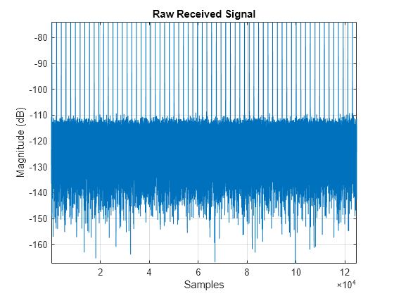
Plot the raw received I/Q signal. The direct path is the strongest return in the datacube. In a bistatic radar geometry, the direct path is shorter than a target path, because the direct path travels directly from the transmitter to the receiver, while the target path travels from the transmitter to the target and then back to the receiver, resulting in a longer overall distance traveled due to the added "leg".
% Visualize raw received signal
timeVec = (0:(size(y,1) - 1))*1/fs;
figure()
plot(timeVec,mag2db(abs(sum(y,2))))
grid on
axis tight
xlabel('Time (sec)')
ylabel('Magnitude (dB)')
title('Raw Received Signal')
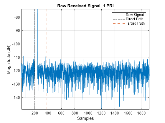
Next, plot the raw received I/Q signal for a single pulse repetition interval (PRI). The purple dot dash line indicates the start index of the direct path. The red dashed line indicates the index of the target return, which is not easily visible within a single PRI. The target will only become apparent after additional signal processing.
% Calculate direct path start sample
[dpRng,dpAng] = rangeangle(poses(1).Position(:),poses(2).Position(:),poses(2).Orientation.');
tDP = range2time(dpRng/2,c);
[~,startIdxDp] = min(abs(timeVec - tDP));

% Calculate target start sample
tgtRng = Rtx + Rrx - dpRng;
tTgt = range2time(tgtRng/2,c);
[~,tgtSampleIdx] = min(abs(timeVec - tTgt));

% Visualize raw received signal including direct path and target sample
% positions
figure()
plot(mag2db(abs(sum(y(startIdx:endIdx,:),2))))
xline(startIdxDp,'-.',SeriesIndex=4,LineWidth=1.5)
xline(tgtSampleIdx + startIdxDp,'--',SeriesIndex=2,LineWidth=1.5)
hold on
grid on
axis tight
xlabel('Samples')
ylabel('Magnitude (dB)')
title('Raw Received Signal, 1 PRI')
legend('Raw Signal','Direct Path','Target Truth')
Create Bistatic Datacube
Build the bistatic datacube. Typically, a bistatic datacube is zero-referenced to the direct path. This means that the target bistatic range and Doppler are relative to the direct path. The bistatic radar in this case is stationary, so no zeroing of Doppler is required. Decrease the number of pulses by 1 to prevent an incomplete datacube in the last PRI.
This example assumes that the transmitter and receiver are time-synchronized, and the positions of the transmitter and receiver are known. All subsequent processing will be performed on the bistatic datacube formed in this section.
% Create bistatic datacube
startIdx = startIdxDp;
numSamples  = round(fs*pri); % Number of range samples
endIdx = startIdx + numSamples - 1;
numPulses = numPulses - 1;
yBi = zeros(numSamples,numElements,numPulses);
for ip = 1:numPulses
    yBi(:,:,ip) = y(startIdx:endIdx,:);
    startIdx = endIdx + 1;
    endIdx = startIdx + numSamples - 1;
end
timeVec = timeVec(1:numSamples*numPulses);
Visualize the bistatic datacube by summing over the antenna elements in the receive array, forming a sum beam at the array broadside. The x-axis is slow time (pulses), and the y-axis is fast-time (samples). The strong direct path return is noticeable. The red dashed line indicates the sample index of the target return relative to the direct path.
% Visualize bistatic datacube
helperPlotBistaticDatacube(yBi,tgtSampleIdx)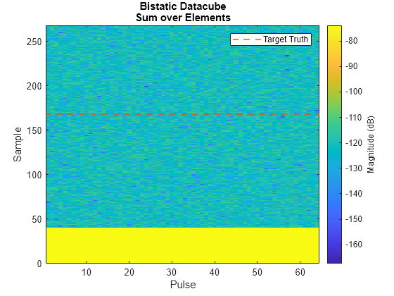
Process Bistatic Datacube
Match Filter and Doppler Process
Perform matched filtering and Doppler processing using the phased.RangeDopplerResponse object. Oversample in Doppler by a factor of 2 and apply a Taylor window with 40 dB sidelobes to improve the Doppler spectrum.
% Perform matched filtering and Doppler processing
rngdopresp = phased.RangeDopplerResponse(SampleRate=fs,...
    Mode='Bistatic', ...
    PropagationSpeed=c, ...
    DopplerFFTLengthSource='Property', ...
    DopplerWindow='Taylor', ...
    DopplerSidelobeAttenuation=40, ...
    DopplerFFTLength=2*numPulses, ...
    PRFSource='Property',PRF=1/pri);
mfcoeff = getMatchedFilter(waveform);
[yBi,rngVec,dopVec] = rngdopresp(yBi,mfcoeff);
The dimensions of the range and Doppler processed datacube are bistatic range-by-number of elements-by-bistatic Doppler.
Calculate the expected bistatic Doppler using the radialspeed function for each leg of the bistatic path.
% Calculate bistatic Doppler
tgtSpdTx = radialspeed(poses(3).Position(:),poses(3).Velocity(:),poses(1).Position(:),poses(1).Velocity(:));
tgtSpdRx = radialspeed(poses(3).Position(:),poses(3).Velocity(:),poses(2).Position(:),poses(2).Velocity(:));
tgtDop = speed2dop((tgtSpdTx + tgtSpdRx),lambda);
Plot the range-Doppler response and show the true bistatic range and Doppler on the image.
% Visualize matched filtered and Doppler processed data
helperPlotRDM(dopVec,rngVec,yBi.*conj(yBi),tgtDop,tgtRng)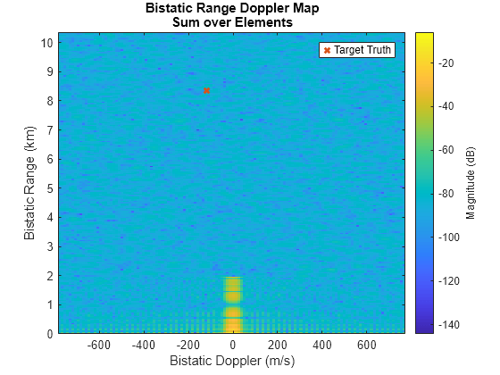
The direct path is still visible as the strong return at 0 range and 0 Doppler. The direct path is localized about 0 Doppler, because the transmitter and receiver are stationary. Note that its range sidelobes extend nearly out to 2 km, and its Doppler sidelobes are visible in the entire Doppler space in those ranges. The target return is still difficult to distinguish due to the influence of the direct path. The true target location is shown as a red x.
Mitigate the Direct Path Interference
The direct path is considered a form of interference. Typically, the direct path return is removed. Mitigation strategies for direct path removal include:
Adding nulls in the known direction of the transmitter
Using a reference beam or antenna
Adaptive filtering in the spatial/time domain
This example removes the direct path by adding nulls in the known direction of the transmitter.
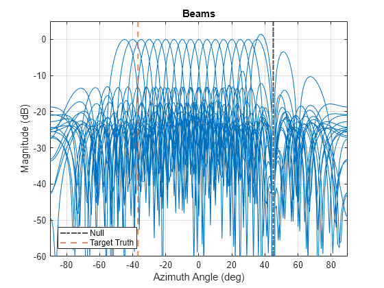
The beamwidth of the receive array is a little over 6 degrees.
% Receiver beamwidth
rxBeamwidth = beamwidth(collector.Sensor,fc)
rxBeamwidth = 6.3600
Specify a series of surveillance beams between -45 and 45 degrees. Space the beams 5 degrees apart in order to minimize scalloping losses.
% Surveillance beams
azSpace = 5;
azAng = -45:azSpace:45;
Null the beams in the direction of the direct path. The angle would be known for this example, since this is a cooperative bistatic case.
% Null angle
nullAng = dpAng;

% Calculate true target angle index
[~,tgtAng] = rangeangle(poses(3).Position(:),poses(2).Position(:),poses(2).Orientation.');
[~,tgtBmIdx] = min(abs(azAng - tgtAng(1)));
Calculate and plot the surveillance beams. The effective receiver azimuth pattern is shown as the thick, solid red line. Note that scalloping losses are minimal. The red dashed line indicates the angle of the target. The purple dot dash line indicates the null angle in the direction of the direct path. The transmitter and receiver in this example are stationary. Thus, the beamforming weights only need to be calculated once.
% Calculate surveillance beams
pos = (0:numElements - 1).*0.5;
numBeams = numel(azAng);
numDop = numel(dopVec);
yBF = zeros(numBeams,numSamples*numDop);
yBi = permute(yBi,[2 1 3]); % <elements> x <bistatic range> x <bistatic Doppler>
yBi = reshape(yBi,numElements,[]); % <elements> x <bistatic range>*<bistatic Doppler>
afAng = -90:90;
af = zeros(numel(afAng),numBeams);
for ib = 1:numBeams
    if ~((azAng(ib) - azSpace) < nullAng(1) && nullAng(1) < (azAng(ib) + azSpace))
        wts = minvarweights(pos,azAng(ib),NullAngle=nullAng);

        % Plot the array factor
        af(:,ib) = arrayfactor(pos,afAng,wts);

        % Beamform
        yBF(ib,:) = wts'*yBi;
    end
end

% Plot beams
helperPlotBeams(afAng,af,nullAng,tgtAng)
% Reshape datacube
yBF = reshape(yBF,numBeams,numSamples,numDop); % <beams> x <bistatic range> x <bistatic Doppler>
yBF = permute(yBF,[2 1 3]); %  <bistatic range> x <beams> x <bistatic Doppler>

% Convert to power
yBF = yBF.*conj(yBF);
Plot the datacube in range-angle space and sum over all Doppler bins. The datacube has now undergone:
Matched filtering
Doppler processing
Beamforming
Nulling of the direct path
The target is now visible. The true target position is indicated by the red x. The deep blue vertical line in the plot below indicates the direct path null. Notice that there is still some leakage from the direct path in the adjacent azimuth bin despite the nulling.
% Plot range-angle after beamforming
helperPlotRAM(azAng,rngVec,yBF,tgtAng(1),tgtRng) 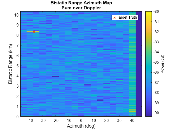
Now plot the datacube in range-Doppler space and sum over all beams. The target is visible and is located where it is expected.
% Plot range-Doppler after beamforming
helperPlotRDM(dopVec,rngVec,yBF,tgtDop,tgtRng)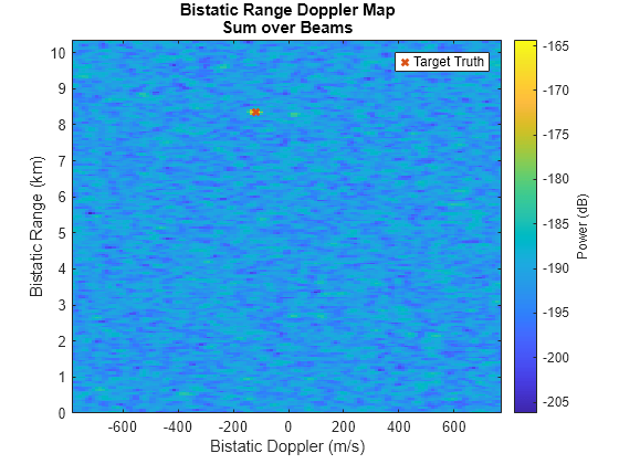
Detect the Target Using 2D CFAR
Perform cell-averaging constant false alarm rate (CA CFAR) processing in 2 dimensions using the phased.CFARDetector2D. The number of training cells ideally totals at least 20 so that the average converges to the true mean, which is easily accomplished in the range dimension. The Doppler dimension has limited bin numbers, so the number of training cells is decreased to 5 on each side.
% Detect using 2D CFAR
numGuardCells    = [10 5]; % Number of guard cells for each side
numTrainingCells = [10 5]; % Number of training cells for each side
Pfa              = 1e-8;  % Probability of false alarm
cfar = phased.CFARDetector2D(GuardBandSize=numGuardCells, ...
    TrainingBandSize=numTrainingCells, ...
    ProbabilityFalseAlarm=Pfa, ...
    NoisePowerOutputPort=true, ...
    OutputFormat='Detection index');
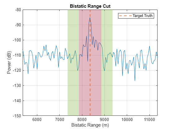
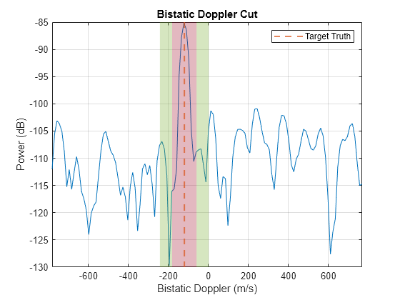
Visualize the range and Doppler cuts for the target. The inner red region shows the guard cells. The outer green region shows the training cells. Note that the training cells do not include contributions from the mainlobe of the target return.
% Visualize range cut
[~,tgtDopIdx] = min(abs(dopVec - tgtDop));
helperPlotCut(yBF(:,tgtBmIdx,tgtDopIdx),rngVec,tgtRng,numGuardCells(1),numTrainingCells(1),'Range','m')
xlim([(tgtRng - 3e3) (tgtRng + 3e3)])
% Visualize Doppler cut
helperPlotCut(yBF(tgtSampleIdx,tgtBmIdx,:),dopVec,tgtDop,numGuardCells(2),numTrainingCells(2),'Doppler','m/s')
Perform two-dimensional CFAR over the beams. Assume that the angle of a detection is the beam azimuth angle.
% Perform 2D CFAR detection
[dets,noise] = helperCFAR(cfar,yBF);
Cluster
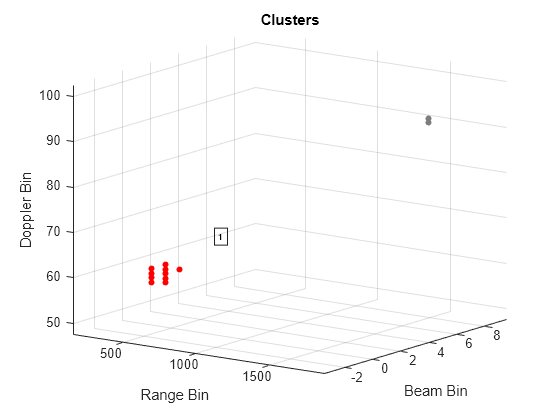
Initialize a DBSCAN (Density-Based Spatial Clustering of Applications with Noise) clustering object. The detections are clustered if they are in adjacent bins.
% Cluster
clust = clusterDBSCAN(Epsilon=1,MinNumPoints=5);
idxClust = clust(dets.');
Plot the clusters. Gray indicates that the false alarms were not clustered.
% Plot clusters
plot(clust,dets.',idxClust);
xlabel('Range Bin')
ylabel('Beam Bin')
zlabel('Doppler Bin')
Return only the highest SNR detection in each cluster.
% Pare down each cluster to a single detection
[detsClust,snrest] = helperDetectionMaxSNR(yBF,dets,noise,idxClust)
detsClust = 3×1
168
3
55
snrest =
22.4959
Estimate Target Parameters
Perform range and Doppler estimation using the phased.RangeEstimator and phased.DopplerEstimator objects, respectively. These objects perform a quadratic fit to refine peak estimation of the target.
% Refine detection estimates in range and Doppler
rangeEstimator = phased.RangeEstimator;
dopEstimator = phased.DopplerEstimator;
rngest = rangeEstimator(yBF,rngVec(:),detsClust);
dopest = dopEstimator(yBF,dopVec,detsClust);
Use the refinepeaks function to improve the azimuth angle estimation.
[~,azest] = refinepeaks(yBF,detsClust.',azAng,Dimension=2);
Output the true and estimated bistatic target range, Doppler, and azimuth. The estimated range, Doppler, and azimuth angle have good agreement with the target truth.
% True target location
Ttrue = table(tgtRng*1e-3,tgtDop,tgtAng(1,:),VariableNames={'Bistatic Range (km)','Bistatic Doppler (m/s)','Azimuth (deg)'});
Ttrue = table(Ttrue,'VariableNames',{'Target Truth'});
disp(Ttrue)
                             Target Truth
    ______________________________________________________________

    Bistatic Range (km)    Bistatic Doppler (m/s)    Azimuth (deg)
    ___________________    ______________________    _____________

          8.3627                  -240.15               -36.79
% Estimated
Test = table(rngest*1e-3,dopest,azest,VariableNames={'Bistatic Range (km)','Bistatic Doppler (m/s)','Azimuth (deg)'});
Test = table(Test,'VariableNames',{'Target Measured'});
disp(Test)
                           Target Measured
    ______________________________________________________________

    Bistatic Range (km)    Bistatic Doppler (m/s)    Azimuth (deg)
    ___________________    ______________________    _____________

          8.3531                  -241.35               -36.573
Plot the detections in range-Doppler space.
% Plot detections
helperPlotRDM(dopVec,rngVec,yBF,tgtDop,tgtRng,dopest,rngest)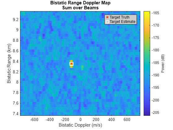
Prepare Data for Tracker
Use the trackerSensorSpec feature to return a sensor configuration appropriate for a bistatic radar system. Set applicable properties based on the previously defined scenario. You can use the sensor spec object as an input sensor specification to a multiSensorTargetTracker (Sensor Fusion and Tracking Toolbox).
sensorSpec = trackerSensorSpec("aerospace","radar","bistatic");
sensorSpec.HasRangeRate                = true;
The receiver must have the target and emitter in its field of view to assume detectability. If not, the tracker may ignore the detection. Set the emitter and receiver field of view properties to 180 degrees in azimuth and 90 degrees in elevation to ensure proper tracking.
% Transmitter properties
txBeamwidth = beamwidth(txarray,fc);
sensorSpec.EmitterPlatformPosition     = poses(1).Position;
sensorSpec.EmitterPlatformOrientation  = poses(1).Orientation;
sensorSpec.EmitterFieldOfView          = [180 90];

% Receiver properties
sensorSpec.ReceiverPlatformPosition    = poses(2).Position;
sensorSpec.ReceiverPlatformOrientation = poses(2).Orientation;
sensorSpec.ReceiverFieldOfView         = [180 90];

% Resolution
% Approximate the angular resolution based on the receiver bandwidth
azres = rxBeamwidth;                         % Azimuth resolution (deg)
rrres = dop2speed(prf/(2*numPulses),lambda); % Range rate resolution (m/s)

% System properties
sensorSpec.AzimuthResolution           = azres;
sensorSpec.RangeResolution             = rngres;
sensorSpec.RangeRateResolution         = rrres;
sensorSpec.FalseAlarmRate              = Pfa
sensorSpec =
  AerospaceBistaticRadar with properties:

    MeasurementMode: "range-angle"

           MaxNumLooksPerUpdate: 1
    MaxNumMeasurementsPerUpdate: 10

           IsReceiverStationary: 1
       ReceiverPlatformPosition: [5000 0 0]      m
    ReceiverPlatformOrientation: [3⨯3 double]
       ReceiverMountingLocation: [0 0 0]         m
         ReceiverMountingAngles: [0 0 0]         deg
            ReceiverFieldOfView: [180 90]        deg
            ReceiverRangeLimits: [0 1e+05]       m
        ReceiverRangeRateLimits: [-500 500]      m/s

           IsEmitterStationary: 1
       EmitterPlatformPosition: [-5000 0 0]     m
    EmitterPlatformOrientation: [3⨯3 double]
       EmitterMountingLocation: [0 0 0]         m
         EmitterMountingAngles: [0 0 0]         deg
            EmitterFieldOfView: [180 90]        deg
            EmitterRangeLimits: [0 1e+05]       m
        EmitterRangeRateLimits: [-500 500]      m/s

           HasElevation: 0
           HasRangeRate: 1
      AzimuthResolution: 6.36     deg
        RangeResolution: 50       m
    RangeRateResolution: 24.38    m/s

    DetectionProbability: 0.9
          FalseAlarmRate: 1e-08
Now that the sensor spec has been defined, use the dataFormat feature with the pre-configured sensor spec object to obtain a data structure for subsequent tracking. Note that the receiver and emitter look azimuths, which are relative to the mount frame of the sensor, are set to 0 degrees, since neither sensor is mechanically scanning.
% Sensor fusion data format
sensorDF = dataFormat(sensorSpec);
sensorDF.ReceiverLookTime              = mean(timeVec);
sensorDF.ReceiverLookAzimuth           = 0;
sensorDF.EmitterLookAzimuth            = 0;
sensorDF.DetectionTime                 = mean(timeVec);
sensorDF.Azimuth                       = azest;
sensorDF.Range                         = rngest;
sensorDF.RangeRate                     = dop2speed(dopest,lambda);
sensorDF.AzimuthAccuracy               = 1./(1.6*sqrt(2*snrest))*azres;
sensorDF.RangeAccuracy                 = sqrt(12)./(sqrt(8*pi^2*snrest))*rngres;
sensorDF.RangeRateAccuracy             = sqrt(6)./(sqrt((2*pi)^2*snrest))*rrres
sensorDF = struct with fields:
ReceiverLookTime: 0.0102
ReceiverLookAzimuth: 0
ReceiverLookElevation: 0
EmitterLookAzimuth: 0
EmitterLookElevation: 0
DetectionTime: 0.0102
Azimuth: -36.5726
Range: 8.3531e+03
RangeRate: -241.1862
AzimuthAccuracy: 0.5926
RangeAccuracy: 4.1097
RangeRateAccuracy: 2.0039
The data is now in a format that is appropriate for a task-oriented tracker like the one demonstrated in the Track Targets Using Asynchronous Bistatic Radars (Sensor Fusion and Tracking Toolbox) example.
Summary
This example outlined a workflow for creating and processing simulated I/Q signals in a cooperative bistatic radar scenario. It illustrated how to import a cone-shaped target using the Antenna Toolbox™. The example involved simulating a bistatic datacube, executing range and Doppler processing, mitigating the direct path interference, and conducting target detection and parameter estimation. Lastly, this example showed how to format data using Sensor Fusion and Tracking Toolbox™ for subsequent tracking using a task-oriented tracker. The demonstrated I/Q simulation and processing techniques can be iteratively applied within a loop to simulate target returns over extended periods.
To further explore waveform-level bistatic simulations, see the Non-Cooperative Bistatic Radar I/Q Simulation and Processing example, which shows how to simulate a passive radar with 2 signals of opportunity.
References
Richards, Mark A. Fundamentals of Radar Signal Processing. 2nd ed. New York: McGraw-Hill education, 2014.
Willis, Nicholas J. Bistatic Radar. SciTech Publishing, 2005.
Helpers
helperPlotScenario
function helperPlotScenario(txPlat,rxPlat,tgtPlat)
% Helper to visualize scenario geometry using theater plotter
%
% Plots:
%    - Transmitter and receiver orientation
%    - Position of all platforms
%    - Target trajectory

% Setup theater plotter
tp = theaterPlot(XLim=[-10 10]*1e3,YLim=[-10 10]*1e3,ZLim=[-10 10]*1e3);
tpFig = tp.Parent.Parent;
tpFig.Units = 'normalized';
tpFig.Position = [0.1 0.1 0.8 0.8];

% Setup plotters:
%   - Orientation plotters
%   - Platform plotters
%   - Trajectory plotters
opTx = orientationPlotter(tp,...
    LocalAxesLength=4e3,MarkerSize=1);
opRx = orientationPlotter(tp,...
    LocalAxesLength=4e3,MarkerSize=1);
plotterTx = platformPlotter(tp,DisplayName='Transmitter',Marker='^',MarkerSize=8,MarkerFaceColor=[0 0.4470 0.7410],MarkerEdgeColor=[0 0.4470 0.7410]);
plotterRx = platformPlotter(tp,DisplayName='Receiver',Marker='v',MarkerSize=8,MarkerFaceColor=[0 0.4470 0.7410],MarkerEdgeColor=[0 0.4470 0.7410]);
plotterTgt = platformPlotter(tp,DisplayName='Target',Marker='o',MarkerSize=8,MarkerFaceColor=[0.8500 0.3250 0.0980],MarkerEdgeColor=[0.8500 0.3250 0.0980]);
trajPlotter = trajectoryPlotter(tp,DisplayName='Target Trajectory',LineWidth=3);

% Plot transmitter and receiver orientations
plotOrientation(opTx,txPlat.Orientation(3),txPlat.Orientation(2),txPlat.Orientation(1),txPlat.Position)
plotOrientation(opRx,rxPlat.Orientation(3),rxPlat.Orientation(2),rxPlat.Orientation(1),rxPlat.Position)

% Plot platforms
plotPlatform(plotterTx,txPlat.Position,txPlat.Trajectory.Velocity,{['Tx, 4' newline 'Element' newline 'ULA']});
plotPlatform(plotterRx,rxPlat.Position,rxPlat.Trajectory.Velocity,{['Rx, 16' newline 'Element' newline 'ULA']});
plotPlatform(plotterTgt,tgtPlat.Position,tgtPlat.Trajectory.Velocity,{'Target'});

% Plot target trajectory
plotTrajectory(trajPlotter,{(tgtPlat.Position(:) + tgtPlat.Trajectory.Velocity(:).*linspace(0,5000,3)).'})
grid('on')
title('Scenario')
view([0 90])
pause(0.1)
end
helperPlotTarget
function helperPlotTarget(hTgtConeAxes,tgtPlat)
% Helper to plot the target structure in the radar scenario

% Setup theater plot
tp = theaterPlot(XLim=(tgtPlat.Position(1) + [-5 5]),YLim=(tgtPlat.Position(2) + [-5 5]),ZLim=(tgtPlat.Position(3) + [-5 5]));
tpFig = tp.Parent.Parent;
tpFig.Units = 'normalized';
tpFig.Position = [0.1 0.1 0.8 0.8];

% Plot platform
plotterTgt = platformPlotter(tp,DisplayName='Target',Marker='o',MarkerSize=8,MarkerFaceColor=[0.8500 0.3250 0.0980],MarkerEdgeColor=[0.8500 0.3250 0.0980]);
plotPlatform(plotterTgt,tgtPlat.Position,tgtPlat.Trajectory.Velocity);
hold on

% Plot cone structure
f = hTgtConeAxes.Children(1).Faces;
verts = hTgtConeAxes.Children(1).Vertices;
patch(tp.Parent,Faces=f,Vertices=verts + tgtPlat.Position,FaceColor=[0.9290 0.6940 0.1250],EdgeColor='none');
grid on

% Label
title('Target in Scenario')
pause(0.1)
end
helperPlotBistaticDatacube
function helperPlotBistaticDatacube(yBi,tgtSampleIdx)
% Helper plots the bistatic datacube

numSamples = size(yBi,1);
numPulses = size(yBi,3);

% Plot bistatic datacube
figure()
imagesc(1:numPulses,1:numSamples,mag2db(abs(squeeze(sum(yBi,2)))))
axis xy
hold on

% Plot target truth line
yline(tgtSampleIdx,'--',SeriesIndex=2,LineWidth=1.5)
ylim([0 tgtSampleIdx + 100])

% Label
xlabel('Pulses')
ylabel('Samples')
title(sprintf('Bistatic Datacube\nSum over Elements'))
legend('Target Truth')

% Colorbar
hC = colorbar;
hC.Label.String = 'Magnitude (dB)';
pause(0.1)
end
helperPlotRDM
function helperPlotRDM(dopVec,rngVec,resp,tgtSpd,tgtRng,dopest,rngest)
% Helper to plot the range-Doppler map
%   - Includes target range and Doppler
%   - Optionally includes estimated range and Doppler
%
% Sums over elements or beams

% Plot RDM
figure
imagesc(dopVec,rngVec*1e-3,pow2db(abs(squeeze(sum(resp,2)))))
hAxes = gca;
axis(hAxes,'xy')
hold(hAxes,'on')

% Plot target truth
plot(hAxes,tgtSpd,tgtRng*1e-3,'x',SeriesIndex = 2,LineWidth=2)

% Optionally plot estimated range and Doppler
if nargin == 7
    plot(hAxes,dopest,rngest*1e-3,'sw',LineWidth=2,MarkerSize=10)
    ylim(hAxes,[tgtRng - 1e3 tgtRng + 1e3]*1e-3)
    legend(hAxes,'Target Truth','Target Estimate',Color=[0.8 0.8 0.8])
else
    ylim(hAxes,[0 tgtRng + 2e3]*1e-3)
    legend(hAxes,'Target Truth');
end

% Colorbar
hC = colorbar(hAxes);
hC.Label.String = 'Power (dB)';

% Labels
xlabel(hAxes,'Bistatic Doppler (m/s)')
ylabel(hAxes,'Bistatic Range (km)')

% Plot title
title(hAxes,'Bistatic Range Doppler Map')

pause(0.1)

end
helperPlotBeams
function helperPlotBeams(afAng,af,nullAng,tgtAng)
% Helper to plot:
%    - Surveillance beams
%    - Null angle
%    - Target angle

% Plot array factor
figure
hArrayAxes = axes;
plot(hArrayAxes,afAng,mag2db(abs(af)),SeriesIndex=1)
hold on
grid on
axis tight
ylim([-60 5])

% Plot array max
azMax = max(mag2db(abs(af)),[],2);
h(1) = plot(hArrayAxes,afAng,azMax,LineWidth=2,SeriesIndex=2);

% Label
xlabel('Azimuth Angle (deg)')
ylabel('Magnitude (dB)')
title('Beams')

% Null angle in direction of direct path
h(2) = xline(nullAng(1),'-.',SeriesIndex=4,LineWidth=1.5);

% Target angle
h(3) = xline(tgtAng(1),'--',LineWidth=1.5,SeriesIndex=2);
legend(h,{'Beam Max','Null','Target Truth'},Location='southwest')
pause(0.1)
end
helperPlotRAM
function helperPlotRAM(azAng,rngVec,yPwr,tgtAng,tgtRng)
% Helper to plot the range-angle map
%   - Includes target range and Doppler
%
% Sums over Doppler

% Plot RAM
figure
imagesc(azAng,rngVec*1e-3,pow2db(abs(squeeze(sum(yPwr,3)))))
axis xy
hold on

% Plot target truth
plot(tgtAng,tgtRng*1e-3,'x',SeriesIndex = 2,LineWidth=2)
ylim([0 tgtRng + 2e3]*1e-3)

% Labels
xlabel('Azimuth (deg)')
ylabel('Bistatic Range (km)')
title(sprintf('Bistatic Range Azimuth Map\nSum over Doppler'))
legend('Target Truth')

% Colorbar
hC = colorbar;
hC.Label.String = 'Power (dB)';
pause(0.1)
end
helperPlotCut
function helperPlotCut(sig,vec,tgtPos,numGuardCells,numTrainingCells,labelChar,unitsChar)
% Helper to plot range and Doppler cuts

% Plot signal
figure
plot(vec,pow2db(abs(squeeze(sig))))
hold on
grid on

% Plot truth
h = xline(tgtPos,'--',SeriesIndex = 2,LineWidth=1.5);

% Guard cells
spacing = vec(end) - vec(end - 1);
ylims = ylim;
x = tgtPos - numGuardCells*spacing;
y = ylims(1);
width = numGuardCells*spacing;
height = ylims(end) - ylims(1);
rectangle(Position=[x y width height],FaceColor=[0.6350 0.0780 0.1840],FaceAlpha=0.3,EdgeColor='none');
x = tgtPos;
rectangle(Position=[x y width height],FaceColor=[0.6350 0.0780 0.1840],FaceAlpha=0.3,EdgeColor='none');

% Training cells
x = tgtPos - (numTrainingCells + numGuardCells)*spacing;
width = numTrainingCells*spacing;
rectangle(Position=[x y width height],FaceColor=[0.4660 0.6740 0.1880],FaceAlpha=0.3,EdgeColor='none');
x = tgtPos + numGuardCells*spacing;
rectangle(Position=[x y width height],FaceColor=[0.4660 0.6740 0.1880],FaceAlpha=0.3,EdgeColor='none');

% Labels
title(['Bistatic ' labelChar ' Cut'])
xlabel(['Bistatic ' labelChar ' (' unitsChar ')'])
ylabel('Power (dB)')
legend(h,{'Target Truth'})
axis tight
pause(0.1)
end
helperCFAR
function [dets,noise] = helperCFAR(cfar,yPwr)
% Helper to determine CUT indices, as well as perform 2D CFAR detection over
% beams

numGuardCells = cfar.GuardBandSize;
numTrainingCells = cfar.TrainingBandSize;

% Determine cell-under-test (CUT) indices
[numSamples,numBeams,numDop] = size(yPwr);
numCellsRng       = numGuardCells(1) + numTrainingCells(1);
idxCUTRng         = (numCellsRng+1):(numSamples - numCellsRng);  % Range indices of cells under test (CUT)
numCellsDop       = numGuardCells(2) + numTrainingCells(2);
idxCUTDop         = (numCellsDop + 1):(numDop - numCellsDop); % Doppler indices of cells under test (CUT)
[idxCUT1,idxCUT2] = meshgrid(idxCUTRng,idxCUTDop);
idxCUT = [idxCUT1(:) idxCUT2(:)].';

% Perform CFAR detection over beams
dets = [];
noise = [];
for ib = 1:numBeams % Perform detection over beams
    [detTmp,noiseTmp] = cfar(squeeze(yPwr(:,ib,:)),idxCUT);
    beamTmp = ib.*ones(1,size(detTmp,2));
    detTmp = [detTmp(1,:); beamTmp; detTmp(2,:)];
    dets = [dets detTmp]; %#ok<AGROW>
    noise = [noise noiseTmp]; %#ok<AGROW>
end
end
helperDetectionMaxSNR
function [detsClust,snrest] = helperDetectionMaxSNR(yPwr,dets,noise,idxClust)
% Helper that outputs the maximum SNR detection in each cluster

idxU = unique(idxClust(idxClust~=-1)); % Unique clusters that are not noise
detsClust = [];
snrest = [];
for iu = 1:numel(idxU)
    idx = find(idxClust == idxU(iu));

    % Find max SNR
    linidx = sub2ind(size(yPwr),dets(1,idx),dets(2,idx),dets(3,idx));
    snrs = yPwr(linidx)./noise(:,idx);
    [~,idxMax] = max(snrs);

    % Save dets
    detsClust = [detsClust [dets(1,idx(idxMax));dets(2,idx(idxMax));dets(3,idx(idxMax))]]; %#ok<AGROW>
    snrest = [snrest yPwr(linidx(idxMax))./noise(:,idx(idxMax))]; %#ok<AGROW>
end
snrest = pow2db(snrest);
end