Introduction to Radar Scenario Clutter Simulation

Configure Scenario for Clutter Generation

Configuration of a radar scenario to simulate surface clutter involves creating a radarScenario object, adding platforms with mounted radars, adding surface objects that define the physical properties of the scenario surface, and enabling clutter generation for a specific radar in the scene.

Select a Radar Model

Clutter generation is performed as part of the scenario detect and receive methods. These methods are used to generate simulated radar detections and IQ signals, respectively. For detections, which consist of measurement-level data along with useful metadata, use the radarDataGenerator. For raw IQ signals, use the radarTransceiver.

This section begins with a radarDataGenerator. Define some typical medium-PRF pulse-Doppler parameters for a side-looking airborne radar. Use a -90 degree mounting yaw angle so the radar faces to the right of the platform and a 10 degree depression angle so the radar is pointed towards the surface. The mounting roll angle can be 0 to indicate no rotation about the antenna boresight. Use a center frequency of 5 GHz, range resolution of 150 m, and a 12 kHz PRF with 64 pulses per coherent processing interval (CPI).

mountAng = [-90 10 0];
fc = 5e9;
rngRes = 150;
prf = 12e3;
numPulses = 64;

The radarDataGenerator is a statistical model that does not directly emulate an antenna pattern. Instead, it has properties that define the field of view and angular resolution. Use 10 degrees for the field of view and angular resolution in each direction. This configuration is comparable to simulating a single mainlobe with no angle estimation.

fov = [10 10];
angRes = fov;

Construct a radarDataGenerator from these parameters. The radar updates once per CPI. The mounting angles point the radar in a broadside direction. Let the field of view and angular resolution equal the beamwidth. Set DetectionCoordinates to 'Scenario' to output detections in scenario coordinates for easier inspection of the results. Calculate the unambiguous range and radial speed and enable range and range-rate ambiguities for the radar. The ambiguities can be calculated with the time2range and dop2speed functions.

c = physconst('lightspeed');
lambda = freq2wavelen(fc);
rangeRateRes = lambda/2*prf/numPulses;
unambRange = time2range(1/prf);
unambRadialSpd = dop2speed(prf/4,lambda);
cpiTime = numPulses/prf;
rdr = radarDataGenerator(1,'No scanning','UpdateRate',1/cpiTime,'MountingAngles',mountAng,...
    'DetectionCoordinates','Scenario','HasINS',true,'HasElevation',true,'HasFalseAlarms',false, ...
    'HasRangeRate',true,'HasRangeAmbiguities',true,'HasRangeRateAmbiguities',true, ...
    'MaxUnambiguousRadialSpeed',unambRadialSpd,'MaxUnambiguousRange',unambRange,'CenterFrequency',fc, ...
    'FieldOfView',fov,'AzimuthResolution',angRes(1),'ElevationResolution',angRes(2), ...
    'RangeResolution',rngRes,'RangeRateResolution',rangeRateRes);

Create a Scenario

The radarScenario object is the top-level manager for the simulation. A radar scenario may be Earth-centered, where the WGS84 Earth model is used, or it may be flat. Use a flat-Earth scenario to enable use of simple kinematic trajectories for the platforms. Set UpdateRate to 0 to let the scenario derive an update rate from the objects in the scenario.

scenario = radarScenario('UpdateRate',0,'IsEarthCentered',false);

Add a radar platform to the scenario. Use a straight-line kinematic trajectory starting 1.5 km up, and moving in the +Y direction at 70 m/s, at a dive angle of 10 degrees. Orient the platform so the platform-frame +X direction is the direction of motion. Use the Sensors property to mount the radar.

rdrAlt = 1.5e3;
rdrSpd = 70;
rdrDiveAng = 10;
rdrPos = [0 0 rdrAlt];
rdrVel = rdrSpd*[0 cosd(rdrDiveAng) -sind(rdrDiveAng)];
rdrOrient = rotz(90).';
rdrTraj = kinematicTrajectory('Position',rdrPos,'Velocity',rdrVel,'Orientation',rdrOrient);
rdrplat = platform(scenario,'Sensors',rdr,'Trajectory',rdrTraj);

Define the Scenario Surface

Physical properties of the scenario surface can be specified by using the scenario landSurface and seaSurface methods to define regions of land and sea surface types. Each surface added to the scene is a rectangular region with an associated radar reflectivity model and reference height. Land surfaces may additionally have associated static terrain data, and sea surfaces may have an associated spectral motion model. If no terrain data or spectral model is used, a surface may be unbounded, allowing for homogeneous clutter generation.

Create a simple unbounded land surface with a constant-gamma reflectivity model. Use the surfaceReflectivity object to create a land reflectivity model and attach the reflectivity model to the surface with the RadarReflectivity parameter. Use a gamma value of -20 dB.

refl = surfaceReflectivity('Land','Model','ConstantGamma','Gamma',-20);
srf = landSurface(scenario,'RadarReflectivity',refl)

srf = 
  LandSurface with properties:

        RadarReflectivity: [1×1 surfaceReflectivityLand]
    ReflectionCoefficient: [1×1 radar.scenario.SurfaceReflectionCoefficient]
          ReflectivityMap: 1
          ReferenceHeight: 0
                 Boundary: [2×2 double]
                  Terrain: []

The ReferenceHeight property gives the constant height of the surface when no terrain is specified, or the origin height to which terrain is referenced if terrain is specified. The ReflectivityMap property is relevant only when a custom reflectivity model is used, and allows different reflectivity curves to be associated to different parts of the surface. The Boundary property gives the rectangular boundary of the surface in two-point form. Elements of Boundary can be +/-inf to indicate the surface is unbounded in one or more directions. Check the boundary of the surface created above to see that it is unbounded in all directions.

srf.Boundary

ans = 2×2

  -Inf   Inf
  -Inf   Inf

Access the SurfaceManager property of the scenario to see the surface objects that have been added, as well as any additional options related to the scenario surface.

scenario.SurfaceManager

ans = 
  SurfaceManager with properties:

    EnableMultipath: 0
       UseOcclusion: 1
           Surfaces: [1×1 radar.scenario.LandSurface]

The UseOcclusion property can be set false to disable line-of-sight occlusions by the surface, such as by terrain.

Enable Clutter Generation

Clutter Generator

Monostatic clutter generation is enabled for a specific radar by using the scenario clutterGenerator method. This method accepts parameter name-value pairs to configure clutter generation. This configuration is performed on a radar-by-radar basis so that multiple radars can be simulated simultaneously with clutter generation settings appropriate for each radar. The clutterGenerator method will return a handle to the ClutterGenerator object.

Reflections from large continuous surfaces are approximated by a set of point scatterers. By default, the ClutterGenerator operates in "uniform" scatterer distribution mode. In this mode, scatterers are placed randomly with a uniform density on the surface. This is a flexible mode that can be used for any surface and radar configuration. See the section below titled "Simulate Smooth Surface Clutter for a Range-Doppler Radar" for a demonstration of a different scatterer distribution mode that can adapt to range-Doppler resolution cells under some scenario constraints. When operating in uniform scatterer distribution mode, the Resolution property specifies the nominal spacing of clutter scatterers used to represent the surface reflection.

The UseBeam property is a logical scalar indicating whether or not automatic mainlobe clutter generation should be used (see the next section titled "Clutter Regions" for more details). The RangeLimit property is used to place an upper bound on the range of clutter generation, which is important for cases when mainlobe clutter generation is being used and has an unbounded footprint.

Create a ClutterGenerator object, enabling clutter generation for the radar created above. Use a Resolution of half the radar's range resolution in order to get a couple of clutter scatterers per range sample. Set UseBeam to true to enable automatic clutter generation within the field of view of the radar. Use a RangeLimit of 12 km, which is just shorter than the unambiguous range.

clutRes = rngRes/2;
clutRngLimit = 12e3;
clut = clutterGenerator(scenario,rdr,'Resolution',clutRes,'UseBeam',true,'RangeLimit',clutRngLimit)

clut = 
  ClutterGenerator with properties:

    ScattererDistribution: "Uniform"
               Resolution: 75
                  Regions: [1×0 radar.scenario.RingClutterRegion]
                  UseBeam: 1
             UseShadowing: 1
               RangeLimit: 12000
                    Radar: [1×1 radarDataGenerator]
               SeedSource: "Auto"

The UseShadowing property is a logical scalar used to enable/disable shadowing (surface self-occlusion). Shadowing is only relevant for surfaces with terrain data or a spectral model.

The clutter generator has two read-only properties. The Radar property stores a handle to the associated radar object, which was passed to the clutterGenerator method. The Regions property contains the set of user-defined "clutter regions".

Clutter Regions

Surface clutter is distributed over the entire range interval starting from the radar altitude and extending to the horizon range (or $$\infty$$ if using a flat-Earth scenario). It is distributed in elevation angle from -90 degrees up to the horizon elevation angle, and over all 360 degrees of azimuth. Finally, surface clutter is distributed in Doppler as a result of platform motion.

There are two options available to designate regions of the surface for clutter generation. The first is automatic mainlobe clutter, which generates clutter inside the footprint of the mainlobe of the radar antenna. This is only possible when the radar being used has a well-defined beam with azimuth and elevation two-sided beamwidths less than 180 degrees. For the radarDataGenerator, the "beam" is actually the field of view defined by the FieldOfView property, the footprint of which consists of contours of constant azimuth and elevation angle. For the radarTransceiver, a conical or fan-shaped beam is assumed based on the array type, and the beam is considered out to 3 dB below the peak gain.

The second option is to use the ringClutterRegion method of the clutter generator to specify a ring-shaped region of the scenario surface within which clutter is to be generated. This type of region is defined by a minimum and maximum ground range (relative to the radar nadir point) and an extent and center angle in azimuth. This region type is useful for capturing sidelobe and backlobe clutter return, mainlobe clutter return outside the 3 dB width, or to generate clutter from any other region of interest, such as at the location of a target platform.

The figure below illustrates these two region types. The beam footprint region is displayed as a magenta ellipse where the beam intersects the ground. Two ring regions are shown, one directly underneath the radar for capturing altitude return, and another for capturing some backlobe clutter return.

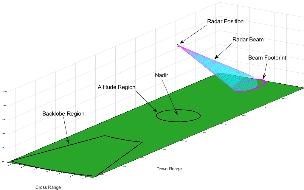
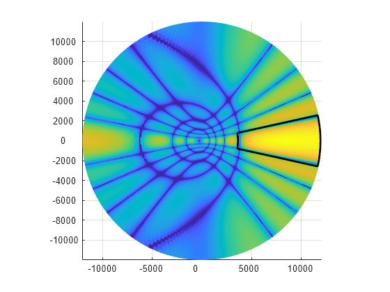
To demonstrate the utility of the customizable ring-shaped regions at capturing clutter return from arbitrary lobes of the antenna pattern, the above geometry is shown again below in a top-down view, with a gain pattern projected onto the ground. Note that a significant backlobe has been encompassed by a ring region. A circular region (which can be achieved by setting the minimum ground range to 0) can be used to capture altitude return. An additional region encompassing the mainlobe is also shown to demonstrate how this can be used to capture more of the mainlobe return, such as from null to null.

The radarDataGenerator is a statistics-based detectability simulator, and only simulates mainlobe detections within the field of view. As such, having UseBeam of the ClutterGenerator set to true is sufficient to completely capture the effect of clutter interference on the detectability of target platforms when using a radarDataGenerator.

Visualize and Run Scenario

Theater Plotter

The theaterPlot object can be used along with a variety of theater plotters to create customizable visual representations of the scenario. Start by creating the theater plot.

tp = theaterPlot;

Now create plotter objects for the scenario surface, clutter regions, and resulting radar detections. The values specified for the DisplayName properties are used for the legend entries.

surfPlotter = surfacePlotter(tp,'DisplayName','Scenario Surface');
clutPlotter = clutterRegionPlotter(tp,'DisplayName','Clutter Region');
detPlotter = detectionPlotter(tp,'DisplayName','Radar Detections','Marker','.','MarkerEdgeColor','magenta','MarkerSize',4);

Now that the scenario, clutter generator, and plotters are configured, use the detect method on the scenario to simulate a single frame and collect detections.

dets = detect(scenario);

Plot the clutter region, which in this case is simply the beam footprint, along with the detection positions. Since the land surface used here is unbounded, the plotSurface call should come last so that the surface plot extends over the appropriate axis limits. The clutterRegionData method on the clutter generator is used to get plot data for the clutter region plotter. Similarly, for the surface plotter, the surfacePlotterData method on the scenario surface manager is used.

plotClutterRegion(clutPlotter,clutterRegionData(clut))
detpos = cell2mat(cellfun(@(t) t.Measurement(1:3).',dets,'UniformOutput',0));
plotDetection(detPlotter,detpos)
plotSurface(surfPlotter,surfacePlotterData(scenario.SurfaceManager))

The detection positions can be seen arranged along radial lines corresponding to the radar's azimuth and Doppler resolution bins. The radarDataGenerator adds noise to the positions of detections, so may return detections with positions that fall outside the beam footprint.

Simulate Clutter IQ Signals

Now you will create a radarTransceiver with similar radar system parameters and simulate clutter at the signal level. The function helperMakeTransceiver is provided to quickly create a transceiver with the desired system parameters.

Define the desired beamwidth. For comparison to the above scenario, simply let the beamwidth equal the field of view that was used.

beamwidth3dB = fov;

The resulting radarTransceiver will use a phased.CustomAntennaElement to approximate a uniform rectangular array with the specified beamwidth, which is recommended to speed up simulations when only a sum beam is needed.

useCustomElem = true;
rdriq = helperMakeTransceiver(beamwidth3dB,fc,rngRes,prf,useCustomElem);

Use the same mounting angles and number of pulses as before.

rdriq.MountingAngles = mountAng;
rdriq.NumRepetitions = numPulses;

Re-create the same scenario, using this new radar model. Start by calling release on System Objects that will be re-used.

release(rdrTraj)
scenario = radarScenario('UpdateRate',0,'IsEarthCentered',false);
platform(scenario,'Sensors',rdriq,'Trajectory',rdrTraj);
landSurface(scenario,'RadarReflectivity',refl);

Enable clutter generation for the radar. This time, disable the beam footprint clutter region in favor of a custom ring-shaped region.

clutterGenerator(scenario,rdriq,'Resolution',clutRes,'UseBeam',false,'RangeLimit',clutRngLimit);

If the clutterGenerator method was called without any output argument, as above, the handle to the constructed ClutterGenerator may still be found with the scenario getClutterGenerator method by passing in a handle to the associated radar.

clut = getClutterGenerator(scenario,rdriq);

After creating the ClutterGenerator, you can use the ringClutterRegion method to create a null-to-null footprint region for clutter generation. Use a simple estimate of the null-to-null beamwidth as about 2.5 times the 3 dB beamwidth, then find the minimum elevation angle to encompass the near edge of the beam, and finally convert that to a minimum ground range for the region.

beamwidthNN = 2.5*beamwidth3dB;
minel = -mountAng(2) - beamwidthNN(2)/2;
minrad = -rdrAlt/tand(minel);

For the max radius parameter, simply find the ground range corresponding to the clutter range limit specified earlier.

maxrad = sqrt(clut.RangeLimit^2 - rdrAlt^2);

The azimuth span will equal the null-to-null beamwidth, and the azimuth center will be 0 degrees since the beam is pointing along the +X direction in scenario coordinates.

azspan = beamwidthNN(1);
azc = 0;
ringClutterRegion(clut,minrad,maxrad,azspan,azc)

ans = 
  RingClutterRegion with properties:

        MinRadius: 3.6213e+03
        MaxRadius: 1.1906e+04
      AzimuthSpan: 25
    AzimuthCenter: 0

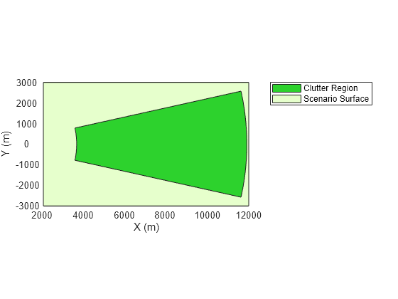
Using the provided helper function, plot the ground-projected antenna pattern along with the ring clutter region you just created. The ring region created above nicely encompasses the entire mainlobe.

helperPlotGroundProjectedPattern(clut)

Run the simulation again for one frame, this time using the scenario receive method to simulate IQ signals.

iqsig = receive(scenario);
PH = iqsig{1};

Since the radarTransceiver used a single custom element, the resulting signal will be formatted with fast-time samples along the first dimension and pulse index (slow time) along the second dimension. This is the phase history (PH) matrix. Plot a DC-centered range-Doppler map (RDM) using the helperPlotRDM function.

figure
helperPlotRDM(PH,rngRes,prf,numPulses)

Use the provided helper function to re-create the theater plot visualization and view the ring clutter region.

helperTheaterPlot(clut)

Simulate Surface Range Profiles for a Scanning Radar

The automatic mainlobe clutter option supports scanning radars. In this section you will re-create the scenario to use a stationary scanning linear array that collects a single pulse per scan position. You will add a few stationary surface targets and view the resulting range profiles.

Start by re-creating the radar object. This time, only pass the azimuth beamwidth to the helper function, which indicates a linear array should be used. The custom element cannot be used for a linear array if the automatic mainlobe clutter option is being used, so that the ClutterGenerator has knowledge of the array geometry. Reduce the range resolution to 75 meters to reduce the clutter power in gate.

useCustomElem = false;
rngRes = 75;
rdriq = helperMakeTransceiver(beamwidth3dB(1),fc,rngRes,prf,useCustomElem);

Set the same mounting angles as used earlier, and configure the transceiver for 1 repetition, which indicates a single pulse per scan position.

numPulses = 1;
rdriq.MountingAngles = mountAng;
rdriq.NumRepetitions = numPulses;

Now configure an electronic sector scan. Set the scanning limits to cover 30 degrees in azimuth, with no elevation scanning. Setting the scan rate to the PRF indicates a single pulse per scan position.

rdriq.ElectronicScanMode = 'Sector';
rdriq.ElectronicScanLimits = [-15 15;0 0];
rdriq.ElectronicScanRate = [prf; 0];

Re-create the scenario and platform. Set the scenario stop time to run 1 full scan. Use a homogeneous unbounded land surface with the same reflectivity model as used earlier.

scenario = radarScenario('UpdateRate',0,'IsEarthCentered',false,'StopTime',30/prf);
platform(scenario,'Sensors',rdriq,'Position',rdrPos,'Orientation',rotz(90).');
landSurface(scenario,'RadarReflectivity',refl);

Enable clutter generation, using only the 3 dB beam footprint for clutter generation.

clutterGenerator(scenario,rdriq,'Resolution',clutRes,'UseBeam',true,'RangeLimit',clutRngLimit);

Add three bright point targets spaced 2 km apart along the cross-range direction at a down-range of 8 km.

tgtRCS = 40; % dBsm
platform(scenario,'Position',[8e3 -2e3 0],'Signatures',rcsSignature('Pattern',tgtRCS));
platform(scenario,'Position',[8e3    0 0],'Signatures',rcsSignature('Pattern',tgtRCS));
platform(scenario,'Position',[8e3  2e3 0],'Signatures',rcsSignature('Pattern',tgtRCS));

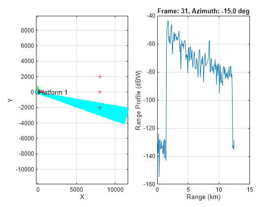
Run the simulation, collecting the range profile at each scan position, and plotting with a scenario overview. Use the info output from receive to record the look angle used by the radar on each frame.

rangeGates = (0:ceil((unambRange-rngRes)/rngRes))*rngRes;
frame = 0;
while advance(scenario)
    frame = frame + 1;
    
    [iqsig,info] = receive(scenario);
    
    lookAng(:,frame) = info.ElectronicAngle;
    rangeProfiles(:,frame) = 20*log10(abs(sum(iqsig{1},2)));
    
    if frame == 1
        % Initial plotting
        ax(1) = subplot(1,2,1);
        helperPlotClutterScenario(scenario,[],[],ax(1))        
        ax(2) = subplot(1,2,2);
        rpHndl = plot(ax(2),rangeGates/1e3,rangeProfiles(:,frame));
        tHndl=title(sprintf('Frame: %d, Azimuth: %.1f deg',frame,lookAng(1,frame)));
        grid on
        xlabel('Range (km)')
        ylabel('Range Profile (dBW)')
    else
        % Update plots
        helperPlotClutterScenario(scenario,[],[],ax(1))
        rpHndl.YData = rangeProfiles(:,frame);
        tHndl.String = sprintf('Frame: %d, Azimuth: %.1f deg',frame,lookAng(1,frame));
    end
    
    drawnow limitrate nocallbacks
end 

Plot the range profiles against range and azimuth scan angle.

figure
imagesc(lookAng(1,:),rangeGates/1e3,rangeProfiles);
set(gca,'ydir','normal')
xlabel('Azimuth Scan Angle (deg)')
ylabel('Range (km)')
title('Clutter Range Profiles (dBW)')
colorbar

The three target signals are barely visible around 8 km range.

Simulate Smooth Surface Clutter for a Range-Doppler Radar

Up till now you have simulated surface clutter using the "uniform" scatterer distribution mode. For flat-Earth scenarios, the radarTransceiver radar model, and smooth surfaces (no terrain or spectral model associated with the surface), a faster range-Doppler-adaptive mode is available which uses a minimal number of clutter scatterers and a more accurate calculation of the clutter power in each range-Doppler resolution cell.

Re-create the radarTransceiver, again with a linear array. The automatic mainlobe region will not be used in this section, so use a custom element to speed things up.

useCustomElem = true;
rdriq = helperMakeTransceiver(beamwidth3dB(1),fc,rngRes,prf,useCustomElem);

This time, instead of scanning, you will just simulate a single frame with 64 pulses, and perform Doppler processing. The NumRepetitions property, along with the specified PRF, determines the Doppler resolution of the adaptive scatterers.

numPulses = 64;
rdriq.MountingAngles = mountAng;
rdriq.NumRepetitions = numPulses;

Create the scenario as before with the simple homogenous surface.

scenario = radarScenario('UpdateRate',0,'IsEarthCentered',false);
landSurface(scenario,'RadarReflectivity',refl);

The radar is again flying in the +Y direction while facing in the +X direction.

release(rdrTraj)
platform(scenario,'Sensors',rdriq,'Trajectory',rdrTraj);

Enable clutter generation. To use the range-Doppler-adaptive scatterers, specify "RangeDopplerCells" for the ScattererDistribution property. To encompass the three targets, use a ring-shaped region with 60 degrees of azimuth span, and the same min/max radius used earlier.

clut = clutterGenerator(scenario,rdriq,'ScattererDistribution','RangeDopplerCells','UseBeam',false,'RangeLimit',clutRngLimit);
ringClutterRegion(clut,minrad,maxrad,60,0);

Add the same three bright targets.

platform(scenario,'Position',[8e3 -2e3 0],'Signatures',rcsSignature('Pattern',tgtRCS));
platform(scenario,'Position',[8e3    0 0],'Signatures',rcsSignature('Pattern',tgtRCS));
platform(scenario,'Position',[8e3  2e3 0],'Signatures',rcsSignature('Pattern',tgtRCS));

Run the simulation for a single frame, form the sum beam, and plot the RDM.

iqsig = receive(scenario);
PH = iqsig{1};
helperPlotRDM(PH,rngRes,prf,numPulses);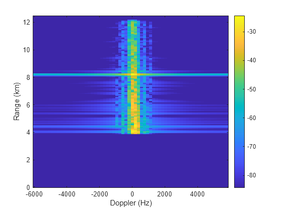

The targets are more visible than in the range-angle case thanks to the Doppler spreading of clutter. With such a large clutter region, the same scenario could be expected to take upwards of 35x longer to simulate with the uniform scatterer distribution.

Clutter from Terrain Data

In the previous sections, you simulated homogeneous clutter from an unbounded flat surface. In this section, you will use a DTED file to simulate clutter return from real terrain data in an Earth-centered scenario. You will collect two frames of clutter return - one with shadowing enabled and one without shadowing, and compare the results.

Start by creating the scenario, this time setting the IsEarthCentered flag to true in order to use a DTED file, which consists of surface height samples over a latitude/longitude grid.

scenario = radarScenario('UpdateRate',0,'IsEarthCentered',true);

Again use the landSurface method, passing in the name of the desired DTED file for the value of the Terrain parameter. The Boundary parameter can be used to constrain the domain of the loaded data. In general, as little of the terrain data should be loaded as needed for the specific application. In this case, you will use a 0.15-by-0.15 degree section of DTED that is referenced to a given latitude-longitude coordinate.

refLLA = [39.43; -105.84];
bdry = refLLA + [0 1;-1/2 1/2]*0.15;

Continue using the same constant-gamma reflectivity model. Use an output argument to get a handle to the created surface object.

srf = landSurface(scenario,'Terrain','n39_w106_3arc_v2.dt1','Boundary',bdry,'RadarReflectivity',refl);

Use the surface height method to place the platform above the reference point at the altitude specified earlier.

srfHeight = height(srf,refLLA);
rdrAlt = srfHeight + rdrAlt;
rdrPos1 = [refLLA; rdrAlt];

In this scenario, the radar will travel in a straight line West at the same speed used earlier.

rdrVelWest = [-rdrSpd 0 0];

Earth-centered scenarios require trajectory information to be specified with waypoints in latitude/longitude/altitude (LLA) format using the geoTrajectory object. Set the ReferenceFrame to ENU, and use the enu2lla function to find the second waypoint corresponding to the desired velocity vector. If the orientation of the platform is not specified, it will be set automatically such that the platform +X direction corresponds to the direction of motion (West). As such, the -90 degree mounting yaw angle will point the radar North.

toa = [0;1]; % Times of arrival at each waypoint
rdrPos2 = enu2lla(rdrVelWest,rdrPos1.','ellipsoid').';
rdrTrajGeo = geoTrajectory('Waypoints',[rdrPos1, rdrPos2].','TimeOfArrival',toa,'ReferenceFrame','ENU');
platform(scenario,'Sensors',rdriq,'Trajectory',rdrTrajGeo);

Create the clutter generator. Surface shadowing is enabled by default.

clut = clutterGenerator(scenario,rdriq,'Resolution',clutRes,'UseBeam',false,'RangeLimit',clutRngLimit);

Create a ring-shaped region with the same parameters as earlier. For Earth-centered scenarios, azimuth angles in scenario coordinates are referenced clockwise from North, so an azimuth center of 0 here still coincides with the radar's look direction.

ringClutterRegion(clut,minrad,maxrad,azspan,azc);

Simulate clutter return for one frame and save the resulting phase history.

iqsig = receive(scenario);
PH_withShadowing = iqsig{1};

The theater plot does not support visualizations of Earth-centered scenarios, so use the provided helper function to show a scenario overview in a local ENU frame. This time, the terrain is plotted along with the radar frame and clutter patches. Notice the shadowed region can be seen in the plot as a gap in the clutter patches (cyan). Those patches are obstructed by other parts of the terrain that are closer to the radar.

helperPlotClutterScenario(scenario)
title('Clutter patches - with terrain shadowing')

To see the difference when shadowing is not used, turn shadowing off, run the simulation for another frame, and save the result.

clut.UseShadowing = false;
iqsig = receive(scenario);
PH_noShadowing = iqsig{1};

Plot the scenario overview and notice that some of the clutter region has been filled in with clutter patches. Notice there are still some gaps visible. This is because clutter patches that are facing away from the radar, such as if they are on the other side of a hill, will never be visible, regardless of the value of the UseShadowing property.

helperPlotClutterScenario(scenario)
title('Clutter patches - without terrain shadowing')

Now to see the effect of shadowing in the RDM, plot the clutter return signals recorded previously side-by-side.

figure
subplot(1,2,1)
helperPlotRDM(PH_withShadowing,rngRes,prf,numPulses)
title('RDM - with terrain shadowing')
subplot(1,2,2)
helperPlotRDM(PH_noShadowing,rngRes,prf,numPulses)
title('RDM - without terrain shadowing')
set(gcf,'Position',get(gcf,'Position')+[0 0 560 0])

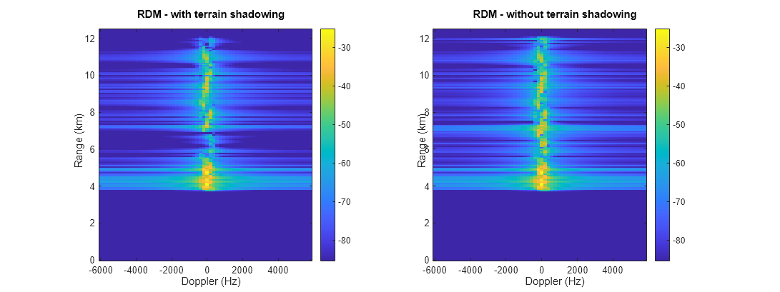
While both cases have "blank" regions due to hills that slope away from the radar, there is also a significant amount of surface return that is visible in the right figure and not visible in the left due to shadowing.

Shadowing is an important phenomenon when simulating clutter return from real surfaces, but it may be disabled for analysis purposes or if not needed.

Conclusion

In this example, you saw how to configure a radar scenario to include clutter return as part of the detect and receive methods, generating clutter detections and IQ signals with the radarDataGenerator and radarTransceiver, respectively. You saw how to define a region of the scenario surface with an associated reflectivity model, and how to specify regions of interest for clutter generation. Surface shadowing is simulated when generating clutter returns from surfaces with terrain, and a faster range-Doppler-adaptive mode can be used for flat-Earth scenarios with smooth surfaces.

Supporting Functions

helperTheaterPlot

function helperTheaterPlot(clut,params)

arguments
    clut
    params.Parent = []
    params.Detections = []
    params.ShowPatches = false
end

if isempty(params.Parent)
    % Make new figure for theater plot
    figure
    tp = theaterPlot('Parent',gca);
else
    % Use specified axes
    cla(params.Parent)
    tp = theaterPlot('Parent',params.Parent);
end

% Find targets
tgts = clut.Scenario.Platforms(2:end);
if ~isempty(tgts)
    tgtPos = cell2mat(cellfun(@(t) t.Position,tgts.','UniformOutput',0));
end

% Get detection positions
if ~isempty(params.Detections)
    detPos = cell2mat(cellfun(@(t) t.Measurement(1:3).',params.Detections,'UniformOutput',0));
end

% Make plotters
if ~isempty(tgts)
    platPlotter = platformPlotter(tp,'DisplayName','Target','Marker','+','MarkerEdgeColor','r');
end
if ~isempty(params.Detections)
    detPlotter = detectionPlotter(tp,'DisplayName','Radar Detections','Marker','.','MarkerEdgeColor','magenta','MarkerSize',4);
end
clutPlotter = clutterRegionPlotter(tp,'DisplayName','Clutter Region','ShowPatchCenters',params.ShowPatches);
surfPlotter = surfacePlotter(tp,'DisplayName','Scenario Surface');

% Do plotting
if ~isempty(tgts)
    plotPlatform(platPlotter,tgtPos);
end
plotHeight = 1;
plotClutterRegion(clutPlotter,clutterRegionData(clut,plotHeight))
if ~isempty(params.Detections)
    plotDetection(detPlotter,detPos)
end
plotSurface(surfPlotter,surfacePlotterData(clut.Scenario.SurfaceManager))

end

helperMakeTransceiver

function rdr = helperMakeTransceiver( bw,fc,rangeRes,prf,useCustomElem )
% This helper function creates a radarTransceiver from some basic system
% parameters.

c = physconst('lightspeed');

rdr = radarTransceiver;

rdr.TransmitAntenna.OperatingFrequency = fc;
rdr.ReceiveAntenna.OperatingFrequency = fc;

rdr.Waveform.PRF = prf;

sampleRate = c/(2*rangeRes);
sampleRate = prf*round(sampleRate/prf); % adjust to match constraint with PRF

rdr.Receiver.SampleRate = sampleRate;
rdr.Waveform.SampleRate = sampleRate;

rdr.Waveform.PulseWidth = 2*rangeRes/c;

if isempty(bw)
    % Use an isotropic element
    rdr.TransmitAntenna.Sensor = phased.IsotropicAntennaElement;
    rdr.ReceiveAntenna.Sensor = phased.IsotropicAntennaElement;
else
    % Get the number of elements required to meet the specified beamwidth
    sinc3db = 0.8859;
    N = round(sinc3db*2./(bw(:).'*pi/180));
    N = flip(N);
    lambda = freq2wavelen(fc,c);
    if numel(N) == 1
        % Use a back-baffled ULA
        array = phased.ULA(N,lambda/2);
        array.Element.BackBaffled = true;
    else
        % Use URA
        array = phased.URA(N,lambda/2);
    end

    if useCustomElem
        % Use a custom element corresponding to the sum beam
        az = -180:.4:180;
        el = -90:.4:90;
        G = pattern(array,fc,az,el,'Type','efield','normalize',false);
        M = 20*log10(abs(G));
        P = angle(G);
        E = phased.CustomAntennaElement('FrequencyVector',[fc-1 fc+1],...
            'AzimuthAngles',az,'ElevationAngles',el,'MagnitudePattern',M,'PhasePattern',P);
        rdr.TransmitAntenna.Sensor = E;
        rdr.ReceiveAntenna.Sensor = E;
    else
        rdr.TransmitAntenna.Sensor = array;
        rdr.ReceiveAntenna.Sensor = array;
    end
end

end

helperPlotGroundProjectedPattern

function helperPlotGroundProjectedPattern( clut )
% Input a ClutterGenerator that has an associated radarTransceiver. Plots
% the clutter regions and ground-projected gain pattern. Assumes a flat
% infinite ground plane at Z=0.

Naz = 360*4;
Nel = 90*4;

% Force update the patch generator sensor data
clut.PatchGenerator.updateSensorData(clut.Platform,clut.Radar,clut.Scenario.SimulationTime,clut.UseBeam);

pos = clut.PatchGenerator.SensorData.Position;
fc = clut.PatchGenerator.SensorData.CenterFrequency;
B = clut.PatchGenerator.SensorData.SensorFrame;
maxGndRng = clut.RangeLimit;

% Get azimuth/elevation grid in scenario coordinates
azScen = linspace(-180,180,Naz);
maxEl = -atand(pos(3)/maxGndRng);
elScen = linspace(-90,maxEl,Nel);

% Convert az/el to sensor frame
[losxScen,losyScen,loszScen] = sph2cart(azScen*pi/180,elScen.'*pi/180,1);
R = B.';
losx = R(1,1)*losxScen + R(1,2)*losyScen + R(1,3)*loszScen;
losy = R(2,1)*losxScen + R(2,2)*losyScen + R(2,3)*loszScen;
losz = R(3,1)*losxScen + R(3,2)*losyScen + R(3,3)*loszScen;
[az,el,~] = cart2sph(losx,losy,losz);
az = az*180/pi;
el = el*180/pi;

% Get gain pattern
sensor = clut.Radar.TransmitAntenna.Sensor;
G = sensor(fc,[az(:) el(:)].');
G = reshape(G,size(az));
G = G/max(G(:));

rtg = -pos(3)./loszScen;
surf(losxScen.*rtg,losyScen.*rtg,zeros(size(az)),20*log10(abs(G)))
axis equal
shading flat
view(0,90)
clim([-60 0])

hold on
for reg = clut.Regions
    helperPlotClutterRegion(reg,pos);
end
hold off

end

helperPlotRDM

function helperPlotRDM( PH,rangeRes,prf,numPulses )
% This helper function forms and plots an RDM from a phase history matrix

c = physconst('lightspeed');

% Form DC-centered RDM and convert to dBW
RDM = fftshift(fft(PH,[],2),2);
RDM = 20*log10(abs(RDM));

% Range and Doppler bins
rngBins = 0:rangeRes:c/(2*prf);
dopBins = -prf/2:prf/numPulses:prf/2-prf/numPulses;

% Plot
imagesc(dopBins,rngBins/1e3,RDM);
set(gca,'ydir','normal')
xlabel('Doppler (Hz)')
ylabel('Range (km)')
mx = max(RDM(:));
if ~isinf(mx)
    clim([mx-60 mx]);
end
colorbar

end