Simulating Radar Datacubes in Parallel

This example uses:

This example shows how to simulate datacubes from an S-band terminal airport surveillance radar in serial and in parallel. The performance of both approaches is compared.

The full functionality of this example requires Parallel Computing Toolbox™.

Create Radar Scenario

First initialize the random number generator for reproducible results.

rng('default')     % Initialize random number generator

Next, specify parameters for an S-band surveillance radar. The radar system will be operating with a bandwidth of 1.5 MHz, a peak power of 1 MW, and a pulse repetition frequency (PRF) of 1 kHz.

% Radar inputs
freq      = 2.8e9; % Frequency (Hz) 
bw        = 1.5e6; % Bandwidth (Hz) 
peakPwr   = 1e6;   % Peak power (W) 
pw        = 1e-6;  % Pulse width (s) 
prf       = 1e3;   % PRF (Hz) 
nf        = 3;     % Noise figure
rdrHgt    = -10;   % Radar height (m)
rdrTilt   = 3;     % Radar tilt angle (deg)
numPulses = 24;    % Number of pulses
rotRate   = 6;     % Rotation rate (deg/s)
fs        = 2*bw;  % Sample rate (Hz) 
arraySize = 16;    % Array size (elements)

This example will investigate processing times with simulated numbers of coherent processing intervals (CPIs) ranging from 20 to 200. Each datacube is of size 3000 range samples-by-16 elements-by-24 pulses. Each CPI simulation is performed 3 times.

numCPIs   = [20:10:100 150 200]; % Number of CPIs
numTrials = 3;                   % Number of trials for each number of CPIs

200 CPIs is equivalent to a scan of about 29 degrees.

pri        = 1/prf;                       % Pulse repetition interval (s)
cpiTime    = numPulses*pri;               % CPI time (s)
numDegrees = (max(numCPIs) - 1)*cpiTime*rotRate % Number of degrees

numDegrees = 28.6560

Define parameters for a target at a starting range of 3 km and with a radar cross section (RCS) of 10 dBsm. A 10 dBsm RCS is representative of a large aircraft. The aircraft will be moving at a speed of 65 m/s.

% Target inputs
tgtRCS    = 10;    % Target RCS (dBsm) 
tgtRng0   = 3e3;   % Target initial range (m)
tgtEl     = -3;    % Target elevation angle (deg)
tgtSpd    = 65;    % Target speed (m/s)
tgtHgt    = tgtRng0.*sind(tgtEl); % Target height (m)

Initialize a radar scenario with an update rate equal to 1 coherent processing interval (CPI).

% Create scenario
maxNumCPIs = max(numCPIs); 
scene = radarScenario('UpdateRate',1/cpiTime,'StopTime',maxNumCPIs*cpiTime);

Create an instance of radarTransceiver to generate IQ. Configure the radarTransceiver such that it is mechanically scanning in a circular pattern with a rotation rate equal to 6 degrees per second. The number of repetitions should be set to the number of pulses in the CPI, which is 24 for this example.

% Create radar sensor
rdr = radarTransceiver('MountingAngles',[0 rdrTilt 0],'NumRepetitions',numPulses, ...
    'MechanicalScanMode','Circular','MechanicalScanRate',rotRate);

Transmit a linear frequency modulated (LFM) waveform.

% Transmit an LFM
rdr.Waveform = phased.LinearFMWaveform('SampleRate',fs,'PRF',prf, ...
    'PulseWidth',pw,'SweepBandwidth',bw);

Update the radar with the other settings from above. Modify the antenna such that it is a uniform linear array (ULA) with 16 elements.

% Configure the radar
rdr.Transmitter.PeakPower = peakPwr; 
lambda = freq2wavelen(freq); 
ula = phased.ULA(arraySize,lambda/2); 
rdr.TransmitAntenna.Sensor = ula;
rdr.Transmitter.Gain = 10; 
rdr.TransmitAntenna.OperatingFrequency = freq;
rdr.ReceiveAntenna.Sensor = ula; 
rdr.ReceiveAntenna.OperatingFrequency = freq;
rdr.Receiver.NoiseFigure = nf;
rdr.Receiver.SampleRate = fs;
rdr.Receiver.Gain = 10;

Attach the radar to a platform.

% Attach radar to a platform
rdrplat = platform(scene,'Position',[0 0 rdrHgt],'Sensor',rdr);

Lastly, create a target platform within the scenario.

% Create target platform 
tgtTraj = kinematicTrajectory('Position',[tgtRng0 0 tgtHgt],'Velocity',tgtSpd*[cosd(tgtEl) 0 sind(tgtEl)]); 
rcsSig = rcsSignature('Pattern',tgtRCS); 
platform(scene,'Trajectory',tgtTraj,'Signature',rcsSig);

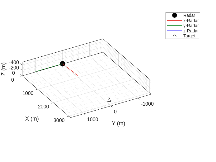
Plot the scenario using theaterPlot. Note that the coordinate system is North-East-Down (NED), so the positive z-axis is down.

% Initialize theater plot
tPlot = theaterPlot('XLimits',[0 3.1e3],'YLimits',[-1.5e3 1.5e3],'ZLimits',[-500 0]);

% Get platform dimensions
profiles = platformProfiles(scene);
dimensions = vertcat(profiles.Dimensions);

% Get platform positions and orientations 
poses = platformPoses(scene);
positions = vertcat(poses.Position);
orientations = vertcat(poses.Orientation);

% Initialize platform and coverage plotters 
orientPlotter = orientationPlotter(tPlot,'DisplayName','Radar',...
    'LocalAxesLength',1e3);
platPlotter = platformPlotter(tPlot,'DisplayName','Target');

% Plot scene 
plotPlatform(platPlotter,positions,dimensions,orientations);
plotOrientation(orientPlotter,rdr.MountingAngles(3),rdr.MountingAngles(2),rdr.MountingAngles(1),rdrplat.Position)

Figure contains an axes object. The axes object with xlabel X (m), ylabel Y (m) contains 5 objects of type line. One or more of the lines displays its values using only markers These objects represent Radar, x-Radar, y-Radar, z-Radar, Target.

Collect Datacubes

Now that the scenario, radar, and target have been configured, generate all the paths for the scenario. The paths include information like:

Path length
Path loss
Reflection coefficient
Angle of arrival/departure (AOA and AOD)
Doppler shift

This information is used by radarTransceiver to simulate returns from targets.

% Advance scenario and collect paths
simTimes = cell(1,maxNumCPIs);
pathsArray = cell(1,maxNumCPIs);
pathGen = helperPaths(scene,'Position',rdrplat.Position);
for ii = 1:maxNumCPIs
    advance(scene);
    simTimes{ii} = scene.SimulationTime;
    pathsArray{ii} = generatePaths(pathGen,rdr);
end

In Serial

To generate datacubes serially, step the radarTransceiver within a loop using the previously computed paths and simulation times for the scenario. The simulation times for each CPI is logged within the elapsedTimeSerial variable. The median of the values in elapsedTimeSerial is taken for each number of CPIs tried.

% Initialize a vector to save off simulation times
elapsedTimeSerial = zeros(numTrials,length(numCPIs));

for iCPI = 1:length(numCPIs)
    for iTrial = 1:numTrials
        % Initialize
        thisNumCPIs = numCPIs(iCPI);
        datacubesSerial = cell(1,thisNumCPIs);

        % Start the clock
        tic; 

        % Step radarTransceiver
        for ii = 1:thisNumCPIs
            datacubesSerial{ii} = rdr(pathsArray{ii},simTimes{ii}); 
        end

        % Get the elapsed time
        elapsedTimeSerial(iTrial,iCPI) = toc;
    end
end

Within the elapsedTimeSerial matrix, the rows represent trials, and the columns represent numbers of CPIs.

% Elapsed time results
numCols = numel(numCPIs) + 1; 
varTypes = repmat("double",1,numCols); 
varNames = ["Serial Trials",compose('%d CPIs',numCPIs)];
elapsedTimeSerialTable = table('Size',[numTrials,numCols],'VariableTypes',varTypes,'VariableNames',varNames); 
elapsedTimeSerialTable(:,1) = num2cell(1:numTrials).';
elapsedTimeSerialTable(1:numTrials,2:numCols) = num2cell(elapsedTimeSerial)

elapsedTimeSerialTable=3×12 table
    Serial Trials    20 CPIs    30 CPIs    40 CPIs    50 CPIs    60 CPIs    70 CPIs    80 CPIs    90 CPIs    100 CPIs    150 CPIs    200 CPIs
    _____________    _______    _______    _______    _______    _______    _______    _______    _______    ________    ________    ________

          1          2.1453     2.4573     3.0859     3.8226     4.7473     5.5038     6.5822      8.011      8.2836      11.885      16.503 
          2          2.3309     2.3244     3.0724     3.9228     4.8138     5.6025      6.637     7.3818      8.4552      11.756      16.819 
          3          3.7697     2.2651     3.1399     3.9556      4.681     5.5928     7.5396     7.5865      8.1003      11.886      17.673

In Parallel

Next, perform the simulation using a parallel worker pool. This example was created using 8 workers. You can change this number based on the number of workers or central processing units (CPUs) in your system.

% Start parallel pool 
parpool;

Starting parallel pool (parpool) using the 'Processes' profile ...
Connected to parallel pool with 8 workers.

The helper helperConfigureRadarTransceiver is used to create replicas of radarTransceiver. This is done to prevent the overhead of passing the preconfigured radarTransceiver class to the workers. In this way, each worker creates a radarTransceiver. Creating the classes on the workers is generally much faster than broadcasting clones. The simulation times for each CPI is logged within the elapsedTimeParallel variable. The median of the values in elapsedTimeParallel is taken for each number of CPIs tried.

% Initialize a vector to save off simulation times
elapsedTimeParallel = zeros(numTrials,length(numCPIs));

for iCPI = 1:length(numCPIs)
    for iTrial = 1:numTrials
        % Initialize 
        thisNumCPIs       = numCPIs(iCPI);
        datacubesParallel = cell(1,thisNumCPIs); 
        thisPathsArray    = pathsArray(1:thisNumCPIs);
        thisSimTimes      = simTimes(1:thisNumCPIs); 

        % Start the clock
        tic; 
        
        % Receive IQ
        parfor ii = 1:thisNumCPIs
            rdrParfor = helperConfigureRadarTransceiver();
            datacubesParallel{ii} = rdrParfor(thisPathsArray{ii},thisSimTimes{ii});
        end

        % Get elapsed time
        elapsedTimeParallel(iTrial,iCPI) = toc;
    end
end

Similar to the elapsedTimeSerial matrix, the rows of elapsedTimeParallel represent trials, and the columns represent numbers of CPIs. Note that the first trial of the first number of CPIs takes much longer than the subsequent trials, because the code needs to be made available to the workers.

% Elapsed time results
varNames = ["Parallel Trials",compose('%d CPIs',numCPIs)];
elapsedTimeParallelTable = table('Size',[numTrials,numCols],'VariableTypes',varTypes,'VariableNames',varNames); 
elapsedTimeParallelTable(:,1) = num2cell(1:numTrials).';
elapsedTimeParallelTable(1:numTrials,2:numCols) = num2cell(elapsedTimeParallel)

elapsedTimeParallelTable=3×12 table
    Parallel Trials    20 CPIs    30 CPIs    40 CPIs    50 CPIs    60 CPIs    70 CPIs    80 CPIs    90 CPIs    100 CPIs    150 CPIs    200 CPIs
    _______________    _______    _______    _______    _______    _______    _______    _______    _______    ________    ________    ________

           1            9.8566    0.94188    2.1701     2.0286     2.0352     2.0714     2.6365     2.6665      3.1966      4.3188      6.0069 
           2           0.91319     0.9755    1.4549     3.5664     1.8023     2.0244     2.3368     2.7509      2.9112      4.6652      5.9557 
           3           0.78305     1.0585    1.3061     2.9374     1.6862     2.2385     2.5841     2.7274      2.8208      4.6443      6.2298

The simulation is now finished. Proceed to shut down the parallel pool.

delete(gcp('nocreate'));

Parallel pool using the 'Processes' profile is shutting down.

Compare Approaches

First compare the resultant datacubes. Note that the two methods create similar results.

% Create a range-Doppler response object
rngdop = phased.RangeDopplerResponse('SampleRate',fs); 
matchFilt = getMatchedFilter(rdr.Waveform); 

% Form a range-Doppler map for a serial datacube
[respS,rngGrid,dopGrid] = rngdop(datacubesSerial{1},matchFilt);

% Form a range-Doppler map for a parallel datacube
respP = rngdop(datacubesParallel{1},matchFilt);

% Range-Doppler map of serial computation
figure
tiledlayout(1,2); 
nexttile;
hAxes = gca; 
helperPlotRDM(hAxes,rngGrid,dopGrid,respS,tgtRng0,'Serial');

% Range-Doppler map of parallel computation
nexttile;
hAxes = gca; 
helperPlotRDM(hAxes,rngGrid,dopGrid,respP,tgtRng0,'Parallel');

Figure contains 2 axes objects. Axes object 1 with title Serial, xlabel Doppler (Hz), ylabel Range (km) contains an object of type surface. Axes object 2 with title Parallel, xlabel Doppler (Hz), ylabel Range (km) contains an object of type surface.

Calculate the median over the trials for each CPI.

% Compute medians of elapsed times
elapsedTimeSerialMedian   = median(elapsedTimeSerial,1);
elapsedTimeParallelMedian = median(elapsedTimeParallel,1);

Compare the elapsed times for simulating datacubes serially and in parallel.

% Plot elapsed times
figure
hAxes = axes; 
hP1   = plot(numCPIs,elapsedTimeSerialMedian,'o');
hold on
hP2   = plot(numCPIs,elapsedTimeParallelMedian,'o'); 

% Plot best fit lines 
helperPlotBestFitLine(hAxes,numCPIs,elapsedTimeSerialMedian,1);
helperPlotBestFitLine(hAxes,numCPIs,elapsedTimeParallelMedian,2);

% Add labels 
grid on
legend([hP1 hP2],'Serial','Parallel','Location','northwest') 
title('Datacube Simulation Times')
xlabel('Number of CPIs')
ylabel('Elapsed Time (sec)')

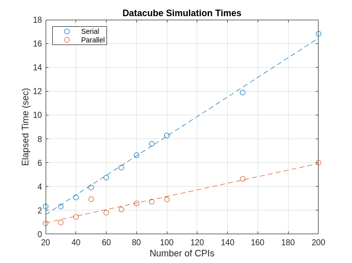
Figure contains an axes object. The axes object with title Datacube Simulation Times, xlabel Number of CPIs, ylabel Elapsed Time (sec) contains 4 objects of type line. One or more of the lines displays its values using only markers These objects represent Serial, Parallel.

The figure shows that there is not much performance improvement for small numbers of CPIs. However, when generating larger numbers of CPIs, the parallel processing simulation time is generally faster.

speedUp = elapsedTimeSerialMedian(end)/elapsedTimeParallelMedian(end);
fprintf('The median parallel processing time is %.2f times faster than the median serial processing time for the %d CPIs case.',speedUp,numCPIs(end));

The median parallel processing time is 2.80 times faster than the median serial processing time for the 200 CPIs case.

Summary

This example showed how to simulate datacubes from an S-band terminal airport surveillance radar serially and in parallel. When generating large numbers of CPIs, parallel processing was shown to improve performance. Parallelizing a simulation can be useful for radar simulations when there is a scanning radar and many CPIs must be generated for a search area.

Helpers

helperConfigureRadarTransceiver

function rdr = helperConfigureRadarTransceiver()
% Helper creates a radarTransceiver for use with parfor

% Radar inputs
freq      = 2.8e9; % Frequency (Hz) 
bw        = 1.5e6; % Bandwidth (Hz) 
peakPwr   = 1e9;   % Peak power (W) 
pw        = 1e-6;  % Pulse width (s) 
prf       = 1e3;   % PRF (Hz) 
nf        = 3;     % Noise figure
rdrTilt   = 3;     % Radar tilt angle (deg)
numPulses = 24;    % Number of pulses
rotRate   = 6;     % Rotation rate (deg/s)
fs        = 2*bw;  % Sample rate (Hz) 
arraySize = 16;    % Array size (elements) 

% Create radar sensor
rdr = radarTransceiver('MountingAngles',[0 rdrTilt 0],'NumRepetitions',numPulses, ...
    'MechanicalScanMode','Circular','MechanicalScanRate',rotRate); 

% Transmit an LFM
rdr.Waveform = phased.LinearFMWaveform('SampleRate',fs,'PRF',prf, ...
    'PulseWidth',pw,'SweepBandwidth',bw); 

% Configure the radar
rdr.Transmitter.PeakPower = peakPwr; 
lambda = freq2wavelen(freq); 
ula = phased.ULA(arraySize,lambda/2); 
rdr.TransmitAntenna.Sensor = ula;
rdr.Transmitter.Gain = 10; 
rdr.TransmitAntenna.OperatingFrequency = freq;
rdr.ReceiveAntenna.Sensor = ula; 
rdr.ReceiveAntenna.OperatingFrequency = freq;
rdr.Receiver.NoiseFigure = nf;
rdr.Receiver.SampleRate = fs;
rdr.Receiver.Gain = 10; 
end

helperPlotRDM

function helperPlotRDM(hAxes,rngGrid,dopGrid,resp,tgtRng,titleStr)
% Helper function to plot range-Doppler map (RDM) 

[~,idxRng] = min(abs(rngGrid - (tgtRng + 1e3)));
hP = pcolor(hAxes,dopGrid,rngGrid(1:idxRng)*1e-3,mag2db(abs(squeeze(sum(resp(1:idxRng,:,:),2)))));
hP.EdgeColor = 'none'; 
xlabel('Doppler (Hz)')
ylabel('Range (km)') 
title(titleStr) 
hC = colorbar; 
hC.Label.String = 'Magnitude (dB)'; 
end

helperPlotBestFitLine

function helperPlotBestFitLine(hAxes,x,y,colorNum)
% Helper function that creates a best fit line

coefficients = polyfit(x,y,1);
xFit = linspace(min(x),max(x),100);
yFit = polyval(coefficients,xFit);
plot(hAxes,xFit,yFit,'--','SeriesIndex',colorNum);
end