Simulating Radar Returns from a Wind Turbine Using Simple Scatterers
Wind is an affordable natural energy resource that is available on land and offshore, but wind turbines can bring significant challenges for radar systems.
Rotating wind turbine blades create interference that manifests as broad-spectrum Doppler frequency shifts. These effects can have major negative impacts on radar systems resulting in target signal-to-noise ratio (SNR) loss, lower probability of detection, higher false alarm rates, and lost tracks. As a result of the proliferation of wind turbines, there have been many studies on how to mitigate the impact on radar through changes in radar hardware, improving wind turbine design to minimize returns, and updates to radar signal processing.
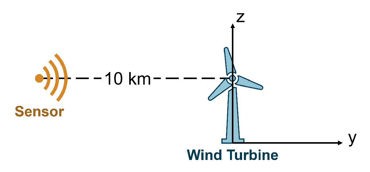
This example demonstrates how to simulate a wind turbine in a radar scenario. The wind turbine return is simulated using a 3-D attributed model in which turbine blades are approximated using simple rectangular plates with known radar cross sections (RCS). IQ data is generated and processed to identify characteristic wind turbine effects in the time-frequency domain.
Define a Radar Scenario
First define an S-band radar system. Set the PRF to 1 kHz. Collect returns from 4000 transmitted pulses.
% Radar parameters
lambda      = 10e-2;        % Wavelength (m)
numPulses   = 4000;         % Number of pulses
prf         = 1e3;          % PRF (Hz)
antBw       = 8;            % Antenna beamwidth (deg)
pulseBw     = 10e6;         % Bandwidth (Hz)
fs          = pulseBw;      % Sampling frequency (Hz)
tpd         = 1e-6;         % Pulse width (sec)
maxRange    = 20e3;         % Maximum range (m)

% Wind turbine parameters
distToRadar = 10e3;         % Range (m)
towerHeight = 48;           % Turbine tower height (m)
Use the bw2rangeres function to estimate the range resolution of the system. Note that the 10 MHz bandwidth provides an approximate range resolution of about 15 meters.
% Calculate range resolution (m)
rangeRes = bw2rangeres(pulseBw)
rangeRes = 14.9896
Create the radar scenario in Cartesian coordinates.
% Create a radar scenario
pri = 1/prf;
dur = pri*(numPulses - 1);
scene = radarScenario('UpdateRate',prf,'StopTime',dur);
Configure a Radar Sensor
Configure the radar sensor. Define a theoretical sinc antenna element with an 8 degree beamwidth. Rotate the sensor such that it is pointing in the direction of the positive y-axis. Limit returns to those between 0 and 20 km.
% Create a radar transceiver
[freq,c] = wavelen2freq(lambda);
ant = phased.SincAntennaElement('Beamwidth',antBw);
rdr = radarTransceiver('MountingAngles',[90 0 0],'RangeLimits',[0 maxRange]);
rdr.TransmitAntenna.Sensor = ant;
rdr.TransmitAntenna.OperatingFrequency = freq;
rdr.ReceiveAntenna.Sensor = ant;
rdr.ReceiveAntenna.OperatingFrequency = freq;
rdr.Receiver.SampleRate = fs;
Set the transmitter and receiver gain to be a value appropriate for the beamwidth. The CosineRectangular option of the beamwidth2gain function is a good approximation for real world antennas.
% Estimate the antenna gain
antennaGain = beamwidth2gain(antBw,'CosineRectangular');
rdr.Transmitter.Gain = antennaGain;
rdr.Receiver.Gain = antennaGain;
Configure the radar sensor's waveform as a linear frequency modulated (LFM) waveform.
% Configure the LFM signal of the radar
rdr.Waveform = phased.LinearFMWaveform('SampleRate',fs,'PulseWidth',tpd, ...
    'PRF',prf,'SweepBandwidth',pulseBw);
Mount the radar sensor to a stationary platform. The sensor will be 10 km from the wind turbine target and mounted at a height of 48 meters equal to the wind turbine tower height.
% Mount radar sensor on a stationary platform
time = 0:pri:(numPulses - 1)*pri;
rdrplatPos = [0 -distToRadar towerHeight];
rdrplat = platform(scene,'Position',rdrplatPos);
rdrplat.Sensors = rdr;
Create a Rotating Wind Turbine
The energy produced by a wind turbine is proportional to the swept area of the blades and to the wind speed. With these considerations in mind, higher efficiency wind turbines tend to employ larger blade rotors and higher towers. This example will model a smaller size wind turbine that is 48 meters tall. The blades are 30 meters long (300 times the wavelength) with a width of 2 meters. Set the rotation rate to 36 degrees per second, meaning that a full rotation of the wind turbine will take 10 seconds. Create the wind turbine with 3 blades spaced 120 degrees apart.
% Wind turbine blade parameters
numBlades   = 3;            % Number of blades
bladeLength = 30;           % Blade length (m)
bladeWidth  = 2;            % Blade width (m)
rotRateDeg  = 36;           % Rotation rate (deg/sec)
rotAng0     = [55 175 295]; % Initial blade rotation angle (deg)

% Wind turbine tower parameters
towerPos = [-bladeWidth;0;towerHeight];
Generally, the tower and the blades are the largest contributing sources for scattering. The nacelle is only a significant scatterer at broadside, and the nosecone is generally insignificant at all angles. For the sake of simplicity, the wind turbine tower and nacelle will not be modeled since the stationary return of the tower can be easily removed using simple Moving Target Indicator (MTI) filtering. This example will only model the moving blades.
There are various ways to model radar returns. At a high level, a complex object can be simulated using an
Isotropic point model, which uses isotropic point scatterers,
2-dimensional attributed model, which uses a combination of point scatterers and simple lines,
3-dimensional attributed model, a composite model that uses simple shapes like cylinders and spheres, or
Electromagnetic (EM) solvers, approximate or full calculation of electromagnetic equations. Examples of EM solvers include Finite-Difference Time-Domain (FDTD) and Method of Moments (MoM). In the case of EM solvers, often a detailed Computer Aided Design (CAD) model is used and is meshed prior to the start of the calculation.

The simulation fidelity increases going from methods 1 to 4. However, as the fidelity increases, so does the associated computational time. This example uses a 3-dimensional attributed model to overcome RCS far field limitations when simulating the entire wind turbine structure at one time.
The general definition of RCS assumes an infinite range and plane wave excitation. The far field can be approximated by a well-known calculation defined as
where is the maximum dimension of the target and is the wavelength. If we were to model the wind turbine tower as a single component, the far field would be at range of about 46 km, which would result in a geometry where the wind turbine was beyond the radar horizon.
% Approximate far field distance in km assuming the entire wind turbine is
% modeled
RkmFarField = 2*towerHeight^2/lambda*1e-3 % Far-field range (km)
RkmFarField =
46.0800
Rhorizon = horizonrange(towerHeight)*1e-3 % Radar horizon (km)Rhorizon = 28.5277
To overcome this issue, the turbine can be modeled using components that are small enough to achieve realistic far field distances. Model the wind turbine using perfectly electrical conducting (PEC), small rectangular plates of length equal to 2 meters. Note that this results in a much smaller far field distance.
% Approximate far field distance in km using smaller components
res         = 2;                  % Rectangular plate length (m)
RkmFarField = 2*res^2/lambda*1e-3 % Far-field range (km)
RkmFarField =
0.0800
To further increase simplicity, the tilt angle of the blades is assumed to be 0. Use helperRcsBladePart to return an rcsSignature object for a single wind turbine rectangular plate component.
% Calculate the RCS of a small rectangular plate
a = bladeWidth;
b = res;
rcsSigBlade = helperRcsBladePart(a,b,c,freq);
Each blade component (rectangular plate) becomes a platform with waypoints, velocities, and orientations based on the rotational movement of the blades. Define the waypoints of the wind turbine components using waypointTrajectory and attach the trajectory to a platform. The geometry of the radar and wind turbine were selected such that the radar is staring at the side of the wind turbine at the height of the wind turbine tower, where blades move towards and away from the radar as the simulation proceeds. This is a worst-case scenario geometry.
Each wind turbine blade is composed of 15 small rectangular plates.
% Determine the number of segments for the wind turbine blade
bladeSegmentHeights = 0:res:bladeLength;
numBladeSegments = numel(bladeSegmentHeights) - 1
numBladeSegments = 15
Create the blades and their trajectories using helperCreateWindTurbine.
% Create wind turbine parts and their trajectories
bladePos = helperCreateWindTurbine(scene,rcsSigBlade,towerHeight,bladeLength,res,rotAng0,rotRateDeg);
Plot the position of the wind turbine scatterers and their trajectories using helperPlotWindTurbine.
% Plot wind turbine movement
helperPlotWindTurbine(rdrplatPos,antBw,distToRadar,bladePos)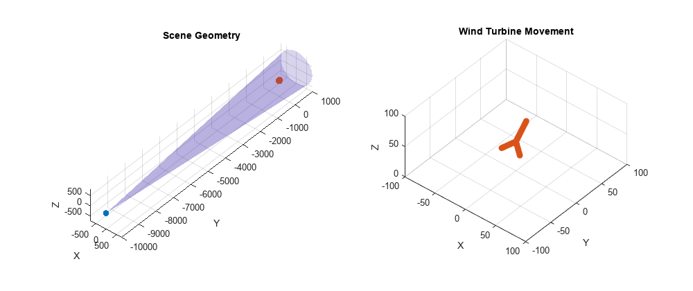
Collect IQ
Collect IQ using the receive method on the radar scenario.
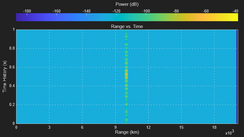
% Initialize output datacube
ib = 0;

timeVec = 0:1/fs:(pri - 1/fs);
rngVec = [0 time2range(timeVec(2:end))];
idx = find(rngVec > maxRange,1,'first');
numSamplesPulse = tpd*fs + 1;
numSamples = idx + numSamplesPulse - 1;
iqsig = zeros(numSamples,numPulses);

% Create range time scope
rti = phased.RTIScope('IQDataInput',true,'RangeLabel','Range (km)', ...
    'RangeResolution',time2range(1/fs), ...
    'TimeResolution',pri,'TimeSpan',1,'SampleRate',fs);

% Collect data
disp('Simulating IQ...')
Simulating IQ...
while advance(scene)
    % Collect IQ
    ib = ib + 1;
    tmp = receive(scene);
    iqsig(:,ib) = tmp{1};
The expected range of the wind turbine is at 10 km. Note that certain orientations of the blade result in a "flash," which is a very bright return. A blade flash occurs when the blade is vertically aligned. The range-time intensity plot shows 3 separate blade flashes.
    % Update scope
    matchingCoeff = getMatchedFilter(rdr.Waveform);
    rti(iqsig(:,ib),matchingCoeff);

    % Update progress
    if mod(ib,500) == 0
        fprintf('\t%.1f %% completed.\n',ib/numPulses*100);
    end
end
	12.5 % completed.
	25.0 % completed.
	37.5 % completed.
	50.0 % completed.
	62.5 % completed.
	75.0 % completed.
	87.5 % completed.
	100.0 % completed.
Investigate Time-Frequency Effects
After collecting the raw IQ data, perform pulse compression using the phased.RangeResponse object.
% Pulse compress and plot
rngresp = phased.RangeResponse('RangeMethod','Matched filter', ...
    'PropagationSpeed',c,'SampleRate',fs);
[pcResp,rngGrid] = rngresp(iqsig,matchingCoeff);
pcRespdB = mag2db(abs(pcResp)); % Convert to dB
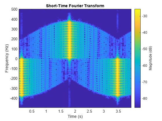
Next, use the short-time Fourier transform (STFT) with a window length of 128 to investigate the time-frequency effects of the rotating wind turbine blades. The plot shows that the blade flashes alternate between negative Doppler, when the blade is moving away from the radar, and positive Doppler, when the blade moves toward the radar. The flashes occur at six times the full rotation period of the turbine due to there being 3 blades present. Negative Doppler and positive Doppler flashes occur three times each during a full rotation period. This example is only transmitting 4000 pulses, which means that only about 40% of the full rotation period is shown. Note that between the bright blade flashes, the magnitude of the spectrum drops considerably, which is as expected.
% Perform STFT and plot
M = 128; % Window length
[maxVal,maxIdx] = max(pcRespdB(:)); % Determine maximum value and its index
[rowIdx,colIdx] = ind2sub(size(pcRespdB),maxIdx); % Identify row index of max return
figure
stft(sum(pcResp((rowIdx-10):(rowIdx+10),:)),prf,'FFTLength',M);
Summary
This example demonstrated how to simulate a wind turbine in a radar scenario using a 3-D attributed model where the turbine blades were simulated using simple rectangular plates with known radar cross sections. IQ data was generated and processed to identify characteristic wind turbine effects in the time-frequency domain. This example can be easily extended to include targets of interest to assess wind turbine performance impacts on metrics like target SNR, probability of detection, and probability of false alarm.
References
Balanis, Constantine A. Advanced Engineering Electromagnetics. 2nd ed. Hoboken, N.J: John Wiley & Sons, 2012.
Energy.gov. “Wind Turbines: The Bigger, the Better.” Accessed June 1, 2023.
Karabayir, Osman, Senem Makal Yucedag, Ahmet Faruk Coskun, Okan Mert Yucedag, Huseyin Avni Serim, and Sedef Kent. “Wind Turbine Signal Modelling Approach for Pulse Doppler Radars and Applications.” IET Radar, Sonar & Navigation 9, no. 3 (March 2015): 276–84.
Krasnov, Oleg A., and Alexander G. Yarovoy. “Radar Micro-Doppler of Wind-Turbines: Simulation and Analysis Using Slowly Rotating Linear Wired Constructions.” In 2014 11th European Radar Conference, 73–76. Italy: IEEE, 2014.
Helpers
helperRcsBladePart
function rcsSigBlade = helperRcsBladePart(a,b,c,fc)
% Helper to return rcsSignature object of a small rectangular PEC plate

% Calculate the RCS of a small rectangular plate
az = -180:1:180;
el = -90:1:90;
rcsBlade = helperRcsPlate(a,b,c,fc,az,el);

% Rotate the rectangular plate such that it is vertical in the y-z plane
el = el + 90;
el = mod(el + 90,180) - 90;
[el,idxSort] = unique(el);
rcsBlade = rcsBlade(idxSort,:);
rcsSigBlade = rcsSignature('Pattern',pow2db(rcsBlade),'Azimuth',az,'Elevation',el);
end
helperRcsPlate
function rcsPat = helperRcsPlate(a,b,c,fc,az,el)
%rcsplate   Radar cross section for flat rectangular plate
%   RCSPAT = helperRcsPlate(A,B,C,FC,AZ,EL) returns the radar cross section
%   (RCS) (in square meters) for a flat rectangular plate at given
%   frequencies. C is a scalar representing the propagation speed (in m/s),
%   and FC is an L-element vector containing operating frequencies (in Hz)
%   at which the RCS patterns are computed.
%
%   AZ are the azimuth angles (in degrees) specified as a Q-element array,
%   and EL are the elevation angles (in degrees) specified as a P-element
%   array. The pairs between azimuth and elevation angles define the
%   directions at which the RCS patterns are computed. This helper assumes
%   a monostatic configuration. HH = VV polarization for this case.
%
%   The flat rectangular plate is assumed to be lying in the x-y plane
%   centered at the origin. Input A is the length of the plate along the
%   x-axis (long side) and B is the width of the plate along the y-axis
%   (short side).
%
%   The RCS calculation assumes a perfectly conducting plate and is an
%   approximation that is only applicable in the optical region, where the
%   target extent is much larger than the wavelength.
%
%   RCSPAT is a P-by-Q-by-L array containing the RCS pattern (in square
%   meters) of the cylinder at given azimuth angles in AZ, elevation angles
%   in EL, and frequencies in FC.

% Reference
% [1] C. A. Balanis, "Advaced Enginnering Electromagnetics", John
%     Wiley&Sons, USA, 1989.

[elg,azg,fcg] = ndgrid(el(:),az(:),fc(:));
lambda = c./fcg;
theta = pi/2 - deg2rad(elg);
phi = deg2rad(azg);

k = 2*pi./lambda; % Wave number

% Balanis
X = k*a/2.*sin(theta).*cos(phi);
idxPos = phi>=0;
Y = zeros(size(X));
Y(idxPos) = k(idxPos)*b/2.*(sin(theta(idxPos)).*sin(phi(idxPos)) + sin(theta(idxPos)));
Y(~idxPos) = k(~idxPos)*b/2.*(sin(theta(~idxPos)).*sin(phi(~idxPos)) - sin(theta(~idxPos)));
rcsPat = 4*pi*(a*b./lambda).^2.*(cos(theta).^2.*sin(phi).^2 + cos(phi).^2) ...
    .*sincFcn(X).^2.*sincFcn(Y).^2 + eps; % TE
end
sincFcn
function y = sincFcn(x)
%sincFcn   Computes the sinc function
%   Y = sincFcn(X) computes the sinc function
%      Y = sin(X)/X.
%   The output Y is the same length as the input X. X is assumed to be in
%   radians.

y = sin(x)./x;
y(isnan(y)) = 1;
end
helperCreateWindTurbine
function bladePos = helperCreateWindTurbine(scene,rcsSigBlade,towerHeight,bladeLength,res,rotAng0,rotRateDeg)
% Helper to create a wind turbine for a radar scenario

% Determine the segment heights and number of segments
bladeSegmentHeights = 0:res:bladeLength;
numBladeSegments = numel(bladeSegmentHeights) - 1;
numBlades = numel(rotAng0);

% Determine the blade segment center points
bladeSegmentCtrs = zeros(3,numBladeSegments);
bladeSegmentCtrs(3,:) = (bladeSegmentHeights(1:end-1) + bladeSegmentHeights(2:end))./2;
rotRateRad = deg2rad(rotRateDeg);

% Simulation time
prf = scene.UpdateRate;
time = scene.SimulationTime:1/prf:scene.StopTime;
numPulses = numel(time);

% Initialize values
platCount = 0;
bladePos = cell(1,numBlades*numBladeSegments);

% Create the moving blades
for ib = 1:numBlades % Loop over blades
    for is = 1:numBladeSegments % Blade segments
        % Blade trajectory
        bladeOrient = zeros(3,3,numPulses);
        bladeWaypoints = zeros(numPulses,3);
        bladeVel = zeros(numPulses,3);
        platCount = platCount + 1;
        for tt = 1:numPulses % Loop over time
            rotAng = rotAng0(ib) + rotRateDeg*time(tt);
            bladeOrient(:,:,tt) = rotx(rotAng);
            bladeWaypoints(tt,:) = bladeOrient(:,:,tt)*bladeSegmentCtrs(:,is);
            bladeVel(tt,:) = cross([rotRateRad;0;0],bladeOrient(:,:,tt)*bladeSegmentCtrs(:,is)); % v = w x r
        end
        % Shift blade waypoints by tower height
        bladeWaypoints(:,3) = bladeWaypoints(:,3) + towerHeight;

        % Create trajectory from waypoints
        bladePos{platCount} = bladeWaypoints;
        traj = waypointTrajectory('SampleRate',prf,'TimeOfArrival',time, ...
            'Waypoints',bladeWaypoints,'Velocities',bladeVel, ...
            'Orientation',bladeOrient);

        % Assign trajectory and rectangular plate RCS to platform
        platform(scene,'Trajectory',traj,'Signatures',rcsSigBlade);
    end
end
end
helperPlotWindTurbine
function helperPlotWindTurbine(rdrplatPos,antBw,distToRadar,bladePos)
% Helper to plot position of wind turbine

% Plot radar
hFig = figure;
currentPos = hFig.Position;
hFig.Position = [currentPos(1) currentPos(2) 1000 currentPos(4)];
tiledlayout(1,2)
hAx1 = nexttile;
co = colororder;
plot3(rdrplatPos(1),rdrplatPos(2),rdrplatPos(3),'o', ...
    'MarkerFaceColor',co(1,:),'MarkerEdgeColor',co(1,:))
hold on
grid on
view([40 40])
axis('equal')
xlabel('X')
ylabel('Y')
zlabel('Z')
title('Scene Geometry')

% Plot radar beam
distBeam = distToRadar*1.1;
coneRad = distBeam.*sind(antBw/2);
[x,y,z] = cylinder([0 coneRad]);
z = z*distBeam;
M = makehgtform('translate',rdrplatPos,'zrotate',pi/2,'yrotate',pi/2);
surf(x,y,z,'Parent',hgtransform('Matrix',M),'LineStyle','none','FaceAlpha',0.2);
hAx2 = nexttile;

% Plot wind turbine
numPulses = size(bladePos{1},1);
for ii = 1:100:numPulses
    x = cellfun(@(x) x(ii,1),bladePos);
    y = cellfun(@(x) x(ii,2),bladePos);
    z = cellfun(@(x) x(ii,3),bladePos);
    if ii == 1
        hTurbine1 = plot3(hAx1,x,y,z,'o', ...
            'MarkerFaceColor',co(2,:),'MarkerEdgeColor',co(2,:));
        hTurbine2 = plot3(hAx2,x,y,z,'o', ...
            'MarkerFaceColor',co(2,:),'MarkerEdgeColor',co(2,:));
        view(hAx2,[40 40])
        axis(hAx2,'equal')
        xlim(hAx2,[-100 100])
        ylim(hAx2,[-100 100])
        zlim(hAx2,[0 100])
        grid(hAx2,'on')
        xlabel(hAx2,'X')
        ylabel(hAx2,'Y')
        zlabel(hAx2,'Z')
        title(hAx2,'Wind Turbine Movement')
    else
        hTurbine1.XData = x;
        hTurbine1.YData = y;
        hTurbine1.ZData = z;
        hTurbine2.XData = x;
        hTurbine2.YData = y;
        hTurbine2.ZData = z;
    end
    pause(0.1)
end

end