Squinted Spotlight Synthetic Aperture Radar (SAR) Image Formation

Radar Configuration

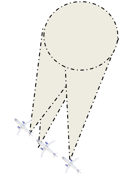
Consider an airborne SAR operating in C-band with a 4 GHz carrier frequency and a signal bandwidth of 50 MHz. This bandwidth yields a range resolution of 3 meters. The radar system collects data at a squint angle of 33 degrees from the broadside as shown in the figure above. The delay corresponds in general to the slant range between the target and the platform. For a SAR system, the slant range will vary over time as the platform traverses a path orthogonal to the direction of antenna beam. This section below focuses on defining the parameters for the transmission waveform. The LFM sweep bandwidth can be decided based on the desired range resolution.

c = physconst('LightSpeed');

Set the SAR center frequency.

fc = 4e9;% Hz

Set the desired range and cross-range resolution to 3 meters.

rangeResolution = 3;% meters
crossRangeResolution = 3;% meters

The signal bandwidth is a parameter derived from the desired range resolution.

bw = c/(2*rangeResolution);

prf = 1000;% Hz
aperture = 4;% sq. meters  
tpd = 3*10^-6; % sec
fs = 120*10^6; % Hz

Configure the LFM signal of the radar.

waveform = phased.LinearFMWaveform('SampleRate',fs, 'PulseWidth', tpd, 'PRF', prf,...
    'SweepBandwidth', bw);

Assume the speed of aircraft is 100 m/s with a flight duration of 4 seconds.

speed = 100;% m/s  
flightDuration = 4;% sec
radarPlatform  = phased.Platform('InitialPosition', [0;-600;500], 'Velocity', [0; speed; 0]);
slowTime = 1/prf;
numpulses = flightDuration/slowTime +1;
eta1 = linspace(0,flightDuration ,numpulses)';

maxRange = 2500;
truncrangesamples = ceil((2*maxRange/c)*fs);
fastTime = (0:1/fs:(truncrangesamples-1)/fs);
% Set the reference range for the cross-range processing.
Rc = 1e3;% meters

Configure the SAR transmitter and receiver. The antenna looks in the broadside direction orthogonal to the flight direction.

antenna = phased.CosineAntennaElement('FrequencyRange', [1e9 6e9]);
antennaGain = aperture2gain(aperture,c/fc); 

transmitter = phased.Transmitter('PeakPower', 1e3, 'Gain', antennaGain);
radiator = phased.Radiator('Sensor', antenna,'OperatingFrequency', fc, 'PropagationSpeed', c);

collector = phased.Collector('Sensor', antenna, 'PropagationSpeed', c,'OperatingFrequency', fc);
receiver = phased.ReceiverPreamp('SampleRate', fs, 'NoiseFigure', 30);

Configure the propagation channel.

channel = phased.FreeSpace('PropagationSpeed', c, 'OperatingFrequency', fc,'SampleRate', fs,...
    'TwoWayPropagation', true);

Scene Configuration

In this example, two static point targets are configured at locations specified below. The entire scene as shown further in the simulation lies ahead of the platform. The data collection ends before the airborne platform is abreast of the target location. All targets have a mean RCS value of 1 meter squared.

targetpos= [900,0,0;1000,-30,0]'; 

targetvel = [0,0,0;0,0,0]';

The squint angle calculation depends on the flight path and center of the target scene which is located at nearly 950 meters in this case.

squintangle = atand(600/950);
target = phased.RadarTarget('OperatingFrequency', fc, 'MeanRCS', [1,1]);
pointTargets = phased.Platform('InitialPosition', targetpos,'Velocity',targetvel);
% The figure below describes the ground truth based on the target
% locations.
figure(1);
h = axes;plot(targetpos(2,1),targetpos(1,1),'*b');hold all;plot(targetpos(2,2),targetpos(1,2),'*r');hold off;
set(h,'Ydir','reverse');xlim([-50 10]);ylim([800 1200]);
title('Ground Truth');ylabel('Range');xlabel('Cross-Range');

SAR Signal Simulation

The following section describes how the system operates based on the above configuration. Specifically, the section below shows how the data collection is performed for a SAR platform. As the platform moves in the cross-range direction, pulses are transmitted and received in directions defined by the squint angle with respect to the flight path. A collection of pulses gives the phase history of the targets lying in the illumination region as the platform moves. The longer the target lies in the illumination region, the better the cross-range resolution for the entire image because the process of range and cross-range focusing is generalized for the entire scene.

rxsig = zeros(truncrangesamples,numpulses);
for ii = 1:numpulses
    % Update radar platform and target position
    [radarpos, radarvel] = radarPlatform(slowTime);
    [targetpos,targetvel] = pointTargets(slowTime);
    
    % Get the range and angle to the point targets
    [targetRange, targetAngle] = rangeangle(targetpos, radarpos);
    
    % Generate the LFM pulse
    sig = waveform();
    % Use only the pulse length that will cover the targets.
    sig = sig(1:truncrangesamples);
    
    % Transmit the pulse
    sig = transmitter(sig);
    
    % Radiate the pulse towards the targets
    sig = radiator(sig, targetAngle);
    
    % Propagate the pulse to the point targets in free space
    sig = channel(sig, radarpos, targetpos, radarvel, targetvel);
    
    % Reflect the pulse off the targets
    sig = target(sig);
    
    % Collect the reflected pulses at the antenna
    sig = collector(sig, targetAngle);
    
    % Receive the signal
    rxsig(:,ii) = receiver(sig);
    
end

kc = (2*pi*fc)/c;
% Compensate for the doppler due to the squint angle
rxsig=rxsig.*exp(-1i.*2*(kc)*sin(deg2rad(squintangle))*repmat(speed*eta1,1,truncrangesamples)).';

Visualize the received signal.

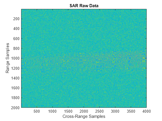
The received signal can now be visualized as a collection of multiple pulses transmitted in the cross-range direction. The plots show the real part of the signal for the two targets. The chirps appear tilted due to the squint angle of the antenna.

imagesc(real(rxsig));title('SAR Raw Data')
xlabel('Cross-Range Samples')
ylabel('Range Samples')

Perform range compression.

The range compression will help achieve the desired range resolution for a bandwidth of 50 MHz.

pulseCompression = phased.RangeResponse('RangeMethod', 'Matched filter', 'PropagationSpeed', c, 'SampleRate', fs);
matchingCoeff = getMatchedFilter(waveform);
[cdata, rnggrid] = pulseCompression(rxsig, matchingCoeff);

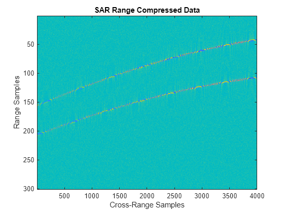
The figure below shows the response after range compression has been achieved on the received signal. The phase histories of the two targets are clearly visible along the cross-range direction and range focusing has been achieved.

imagesc(real(cdata(800:1100,:)));title('SAR Range Compressed Data')
xlabel('Cross-Range Samples')
ylabel('Range Samples')

Azimuth Compression

There are multiple techniques to process the cross-range data and get the final image from the SAR raw data once range compression has been achieved. In essence, the range compression helps achieve resolution in the fast-time or range direction and the resolution in the cross-range direction is achieved by azimuth or cross-range compression. Range Migration algorithm for squint case has been demonstrated in this example. The azimuth focusing needs to account for the squint induced due to antenna tilt.

rma_processed = helperSquintRangeMigration(cdata,fastTime,fc,fs,prf,speed,numpulses,c,Rc,squintangle);

Visualize the final SAR image.

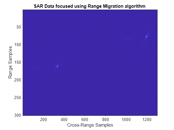
Plot the focused SAR image using the range migration algorithm. Only a section of the image formed via the range migration algorithm is shown to accurately point the location of the targets. The range migration as shown by [1], [2] and [3] provides theoretical resolution in the cross-track as well as along-track direction.

figure(2);
imagesc(abs(rma_processed(2300:3600,1100:1400).'));
title('SAR Data focused using Range Migration algorithm ') 
xlabel('Cross-Range Samples') 
ylabel('Range Samples')

Summary

This example shows how to simulate and develop Squint mode Spotlight SAR processing leveraging a LFM signal in an airborne data collection scenario. The example also demonstrates image generation from the received signal via modified range migration algorithm to handle the effect due to squint.

References

Appendix

Range Migration Algorithm

function azcompresseddata = helperSquintRangeMigration(sigData,fastTime,fc,fs,prf,speed,numPulses,c,Rc,squintangle)

This function demonstrates the range migration algorithm for imaging the side looking synthetic aperture radar. The pulsed compressed synthetic aperture data is considered in this algorithm.

Set the range frequency span.

frequencyRange = linspace(fc-fs/2,fc+fs/2,length(fastTime));
krange = 2*(2*pi*frequencyRange)/c;

Set the cross-range wavenumber.

kaz = 2*pi*linspace(-prf/2,prf/2,numPulses)./speed;

Generate a matrix of the cross-range wavenumbers to match the size of the received two-dimensional SAR signal

kc = 2*pi*fc/3e8;
kazimuth = kaz.';
kus=2*(kc)*sin(deg2rad(squintangle));
kx = krange.^2-(kazimuth+kus).^2;

The wavenumber has been modified to accommodate shift due to squint and achieve azimuth focusing.

thetaRc = deg2rad(squintangle);
kx = sqrt(kx.*(kx > 0));

kFinal = exp(1i*(kx.*cos(thetaRc)+(kazimuth).*sin(thetaRc)).*Rc);
kfin = kx.*cos(thetaRc)+(kazimuth+kus).*sin(thetaRc);

Perform a two-dimensional FFT on the range compressed signal.

sdata =fftshift(fft(fftshift(fft(sigData,[],1),1),[],2),2);

Perform bulk compression to get the azimuth compression at the reference range. Perform filtering of the 2-D FFT signal with the new cross-range wavenumber to achieve complete focusing at the reference range and as a by-product, partial focusing of targets not lying at the reference range.

fsmPol = (sdata.').*kFinal;

Perform Stolt Interpolation to achieve focusing for targets that are not lying at the reference range

stoltPol = fsmPol;
for i = 1:size((fsmPol),1)
    stoltPol(i,:) = interp1(kfin(i,:),fsmPol(i,:),krange(1,:));
end
stoltPol(isnan(stoltPol)) = 1e-30;

azcompresseddata = ifftshift(ifft2(stoltPol),2);

end

References

Cafforio, C., C. Prati, and F. Rocca. "SAR data focusing using seismic migration techniques." IEEE Transactions on Aerospace and Electronic Systems, 27(2), 1991, pp.194–207. https://doi.org/10.1109/7.78293.
Soumekh, M. Synthetic Aperture Radar Signal Processing with MATLAB Algorithms. John Wiley & Sons, 1999.
Stolt, R. H. "Migration by Fourier Transform Techniques." Geophysics, 1978, 43, pp. 23–48.