Rat-Race Coupler - Visualize and Analyze

This example shows you how to create, visualize, and analyze a Rat-Race Coupler.

Create a rat-race coupler with default properties.

ratrace = couplerRatrace

ratrace = 
  couplerRatrace with properties:

      PortLineLength: 0.0186
       PortLineWidth: 0.0050
    CouplerLineWidth: 0.0030
       Circumference: 0.1110
              Height: 0.0016
           Substrate: [1×1 dielectric]
           Conductor: [1×1 metal]
          IsShielded: 0

View the coupler.

show(ratrace)

Figure contains an axes object. The axes object with title couplerRatrace element, xlabel x (mm), ylabel y (mm) contains 8 objects of type patch, surface. These objects represent PEC, feed, Teflon.

Plot the charge distribution at 5 GHz.

charge(ratrace, 5e9)

Figure contains an axes object. The axes object with title Charge distribution, xlabel x (m), ylabel y (m) contains 4 objects of type patch.

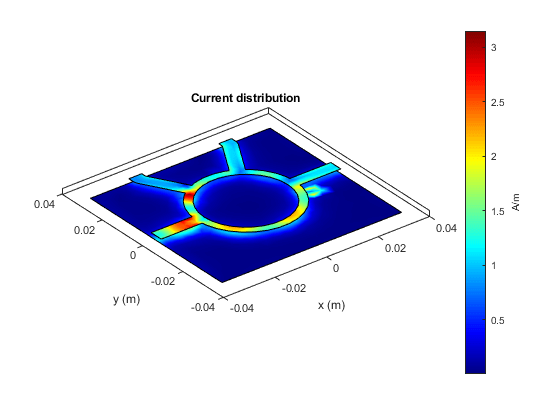
Plot the current distribution at 5 GHz.

figure
current(ratrace, 5e9)

Figure contains an axes object. The axes object with title Current distribution, xlabel x (m), ylabel y (m) contains 4 objects of type patch.

Calculate and plot the s-parameters.

spar = sparameters(ratrace,linspace(1e9,5e9,200),'SweepOption','interpWithGrad')

spar = 
  sparameters with properties:

      Impedance: 50
       NumPorts: 4
     Parameters: [4×4×200 double]
    Frequencies: [200×1 double]

rfplot(spar)

$Figure contains an axes object. The axes object with xlabel Frequency (GHz), ylabel Magnitude (dB) contains 16 objects of type line. These objects represent dB(S_{11}), dB(S_{21}), dB(S_{31}), dB(S_{41}), dB(S_{12}), dB(S_{22}), dB(S_{32}), dB(S_{42}), dB(S_{13}), dB(S_{23}), dB(S_{33}), dB(S_{43}), dB(S_{14}), dB(S_{24}), dB(S_{34}), dB(S_{44}).$

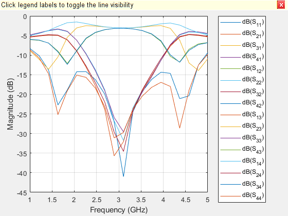
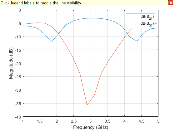
figure
rfplot(spar,[2 3],1)

$Figure contains an axes object. The axes object with xlabel Frequency (GHz), ylabel Magnitude (dB) contains 2 objects of type line. These objects represent dB(S_{21}), dB(S_{31}).$