Circuit Model Extraction of a RF Filter

Open Live Script

This example demonstrates how to create a measuredFilfter object used for computing the Coupling Matrix, using a circuit modeling extraction of the measured Touchstone data file for a 8 pole dielectric resonator filter. The filter has a center frequency at 2114.6528 MHz, a bandwidth of 9.601 MHz and a filter order of 8.

The extracted coupling matrix can be directly compared to the golden reference coupling matrix obtained via filter synthesis. The differences between these matrices can be used to direct what mechanical adjustments should be made to the actual filter to obtain a response that matches the filter response of the golden reference synthesis model. This process can be readily incorporated into the filter prototyping stage of filter design to obtain a desired electrical response. This technique can be used for microwave filters such as cavity, printed, interdigital, combline, and hairpin filters, etc. The extracted models will allow you to characterize filter performance at the individual resonator level rather than at the macro level (network parameters) where simply the filter is described by a black box model.

Read and plot measured filter data

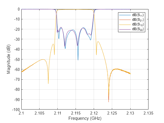
Read and plot the measured S-parameters from the touchstone file FILTER_8.s2p.

It is always recommended that the data used comes from a test setup with proper 2-port network analyzer calibration that extends through the cables. The S-parameter data should be collected over a frequency data range so that both an appropriate amount of passband and rejection band data can be supplied for the model extraction process.

S_measured = sparameters('FILTER_8.s2p');
rfplot(S_measured)
hold on

$Figure contains an axes object. The axes object with xlabel Frequency (GHz), ylabel Magnitude (dB) contains 4 objects of type line. These objects represent dB(S_{11}), dB(S_{21}), dB(S_{12}), dB(S_{22}).$

Create `measuredFilter` object

Create the overall extracted model object, measuredFilter, using each of the following:

an S-parameter object, S_measured
the estimated center frequency, 2114.86235 MHz
filter order, 8, and,
bandwidth, 9.601 MHz.

obj = measuredFilter(Sparameters=S_measured,...
    BandWidth=9.601e6,...
    CenterFrequency=2114.6528e6,...
    FilterOrder=8)

obj = 
  measuredFilter with properties:

            Sparameters: [1x1 sparameters]
            FilterOrder: 8
        CenterFrequency: 2.115 GHz
              BandWidth: 9.601 MHz

   Analysis Results
           LowPassPoles: [0x0 table]
             ResidueY11: [0x0 table]
             ResidueY22: [0x0 table]
             ResidueY12: [0x0 table]
             ResidueY21: [0x0 table]
         CouplingMatrix: [0x0 table]
          QualityFactor: [0x0 table]

Extract residues/poles and calculate the Transversal Coupling Matrix values

From the measuredFilter object, the poles and residues can be determined and subsequently be used to calculate the ‘N+2’ transversal coupling matrix.

[ResidueY11Table, ResidueY12Table] = residue(obj);
cmat = transversalMat(obj)

cmat=10×10 table
               Source        1            2           3            4           5          6           7          8         Load   
              ________    ________    _________    ________    _________    _______    ________    _______    _______    _________

    Source           0     0.33703      0.43742    -0.35247      0.49909     -0.015    -0.43245    0.06074    0.44035            0
    1          0.33703    -0.87462            0           0            0          0           0          0          0      0.36002
    2          0.43742           0      -1.1147           0            0          0           0          0          0    -0.053119
    3         -0.35247           0            0     0.89951            0          0           0          0          0      0.36409
    4          0.49909           0            0           0       1.2532          0           0          0          0    0.0089125
    5           -0.015           0            0           0            0    -1.1939           0          0          0      0.55757
    6         -0.43245           0            0           0            0          0    -0.37421          0          0      0.46244
    7          0.06074           0            0           0            0          0           0     1.2204          0      0.55866
    8          0.44035           0            0           0            0          0           0          0    0.31806      0.45561
    Load             0     0.36002    -0.053119     0.36409    0.0089125    0.55757     0.46244    0.55866    0.45561            0

The ‘extended’ coupling matrix has an extra pair of rows and columns which surround the ‘core’ N x N coupling matrix comprising of N resonant nodes. These extra row and column pairs represent the input and output couplings from the source and load termination to the resonant nodes in the core matrix.

Perform canonical matrix rotations

To transform the transversal coupling matrix into a desirable canonical or folded format, one can perform a series of similarity transforms on the extracted transversal coupling matrix contained in the measuredFilter object, obj. The sequence of matrix rotations are loaded from the mat file, 'mat_rot_8p.mat'.

matrix_index = load('mat_rot_8p.mat');
cmrot = canonicalCouplingMat(obj, matrix_index.matrix_index);

Calculate Q-factor

Calculate the unloaded resonantor quality factor of the measuredFilter object, obj.

Qutable = qualityfactor(obj);

Coupling Matrix transformation

To realize a given filter topology, the extracted canonical or folded coupling matrix will need to be further transformed for realization of transmission zero producing subnetworks. A Gram-Schmidt based method permits one to create a target coupling matrix realization via an optimization process. Typically one would specify a step size of 0.125 and 2500 iterations to achieve a desired coupling matrix configuration.

canon_rot = diag([0 ones(1,obj.FilterOrder) 0])+ ...
    diag(ones(1,obj.FilterOrder+1),1)+diag(ones(1,obj.FilterOrder+1),-1);
[CoupMatrix, Conv] = obj.optimize("Rotation",canon_rot,...
    "NumIterations",2500,"StepSize",0.125);

Compute and plot S-parameters

Calculate the S-parameters of the extracted circuit model obj.

S_calc = sparameters(obj);

Plot the S-parameters from the extracted circuit model, obj, over the original measured frequency range.

rfplot(S_calc,'--')

$Figure contains an axes object. The axes object with xlabel Frequency (GHz), ylabel Magnitude (dB) contains 8 objects of type line. These objects represent dB(S_{11}), dB(S_{21}), dB(S_{12}), dB(S_{22}).$

References

T. Reeves and J. Yanamadala, "Circuit Model Extraction of Coupled-Resonator Filters and Multiplexers Via Direct Use of S-parameter AAA Fitting," 2024 IEEE International Microwave Filter Workshop (IMFW), Cocoa Beach, FL, USA, 2024, pp. 143-146, doi: 10.1109/IMFW59690.2024.10477140.