Design and Analyze Transmission Line in Shielded Enclosure

Open Live Script

This example shows how to design and analyze a transmission line with a shielded enclosure. PCBs often experience unwanted problems such as electromagnetic interference (EMI) leading to performance degradation and failure. This might affect other sensitive electronics due to outgoing EMI. In an ideal world, a shield would completely block off these EMI and ensure that strong signals cannot escape. A microstrip enclosed in a Faraday shield is designed and analyzed using Finite Element Method (FEM). This example also examines an impact of the height of a shielding box and the added metal where a pin from a coax can sit on.

Prerequisites

The example requires the Integro-Differential Modeling Framework for MATLAB add-on. To enable the add-on:

In the Home tab Environment section, click on Add-Ons. This opens the add-on explorer. You need an active internet connection to download the add-on.
Search for Integro-Differential Modeling Framework for MATLAB and click Install
To verify if the download is successful, run matlab.addons.installedAddons in your MATLAB® session command line.

Create Variables

Set a designed frequency and a range of frequency.

Centerfreq = 2e9;
freq = sort([linspace(1e9,3e9,20),2e9]);

Design of Microstrip

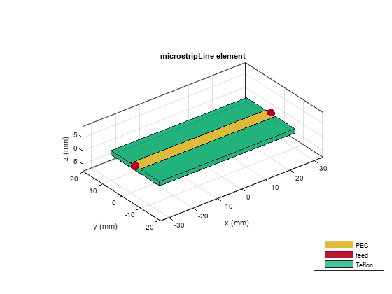
Use the design function on the microstripLine object to create a microstrip at the desired frequency. The default substrate for a microstrip is Teflon.

mline = design(microstripLine,Centerfreq);

Visualize the microstrip.

figure
show(mline)

Figure contains an axes object. The axes object with title microstripLine element, xlabel x (mm), ylabel y (mm) contains 6 objects of type patch, surface. These objects represent PEC, feed, Teflon.

Use the sparameters function to compute the S-parameters in the frequency range of 1 - 3 GHz.

spar1 = sparameters(mline,freq);

Plot the S-parameters of the microstrip.

figure
rfplot(spar1,1);

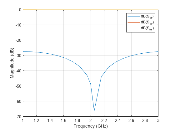
$Figure contains an axes object. The axes object with xlabel Frequency (GHz), ylabel Magnitude (dB) contains 3 objects of type line. These objects represent dB(S_{11}), dB(S_{12}), dB(S_{21}).$

The return coefficient is below -30 dB over the frequency range of 1 - 3 GHz.

Add Metal Shield

Add a 61.8 mm-by-25.6 mm-by-10 mm PEC shielded box to the transmission line. A shield always covers all four sides of a microstrip. Move the shield in z-direction to align its bottom to the ground plane. A microstrip is excited by a coaxial wave port with a characteristic impedance of 50 ohms derived from the outer or inner diameters and the dielectric constant of waveguide region.

mline.IsShielded = true;
mline.Shielding.Height = 10e-3;
mline.Shielding.Center = [0 0 0.5*mline.Shielding.Height];

Visualize the microstrip.

figure
show(mline)

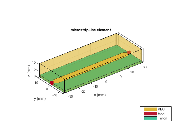
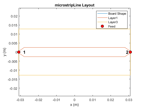
Display the layout of the microstrip. Additional metals are added tapering out from the coax wave port with a width equal to coax inner diameter to the trace of a microstrip. Use PinFootprint and PinLength properties in Connector to determine the shape and length of the added metal for placement of a coax pin . This allows to examine a match between the coax and the borad.

figure
layout(mline)

Impact of Added Metal on S-parameters

Set a range of length of added metal from 0.5 mm to 2 mm.

pinLength = (0.5:0.5:2)*1e-3;

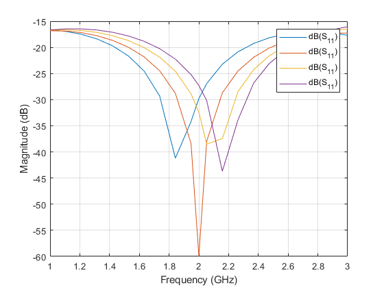
Analyze the impact of the length of added tapered metals on the S-parameters. Use the sparameters function to calculate the S-parameters in the frequency range of 1 - 3 GHz.

for i = 1:numel(pinLength)
   mline.Connector.PinLength = pinLength(i);
   spar2(i) = sparameters(mline,freq); %#ok<SAGROW>
end

Plot the S-parameters of the microstrip with the shield.

figure
rfplot(spar2(1),1,1)
hold on
for i = 2:numel(spar2)
   rfplot(spar2(i),1,1);
end

Impact of Shielding Height on S-parameters

Set the range for the shielding height from 4 mm to 20 mm.

shHeight = (4:4:20)*1e-3;

Set the length of added tapered metal to 1 mm.

mline.Connector.PinLength = 1e-3;

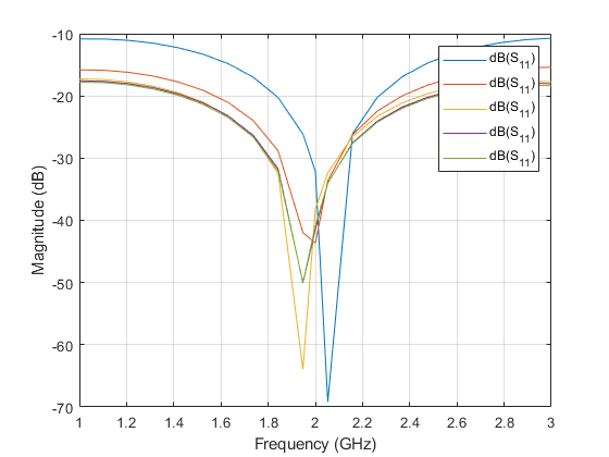
Analyze th impact of the shielding height on the S-parameters. Use the sparameters function to calculate the S-parameters in the frequency range of 1 - 3 GHz.

for i = 1:numel(shHeight)
   mline.Shielding.Height = shHeight(i);
   mline.Shielding.Center = [0 0 0.5*shHeight(i)];
   spar3(i) = sparameters(mline,freq); %#ok<SAGROW>
end

Plot the S-parameters of the microstrip with the shield.

figure
rfplot(spar3(1),1,1)
hold on
for i = 2:numel(spar3)
   rfplot(spar3(i),1,1);
end

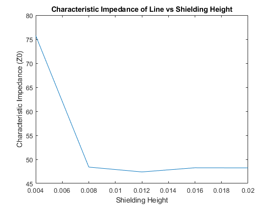
Impact of Shielding Height on Characteristics Impedance

Set the reference impedance.

fcIdx = find(freq==2e9);
ZRef = 50;

Calculate the characteristic impedance of the line from the reflection and transmission coefficients.

for i = 1:numel(spar3)
    s11 = (rfparam(spar3(i),1,1));
    s21 = (rfparam(spar3(i),2,1));
    % Characteristic impedance of the line
    Zlin = ((1+s11(fcIdx)).^2 - s21(fcIdx).^2)./((1-s11(fcIdx)).^2 - s21(fcIdx).^2);
    Z0h(i) = sqrt(ZRef^2*Zlin); %#ok<SAGROW>
end

Plot the characteristics impedance of the microstrip with the shield.

figure
plot(shHeight,abs(Z0h))
xlabel('Shielding Height')
ylabel('Characteristic Impedance (Z0)')
title('Characteristic Impedance of Line vs Shielding Height')