Expected Shortfall (ES) Backtesting Workflow Using Simulation
This example shows an expected shortfall (ES) backtesting workflow using the esbacktestbysim object. The tests supported in the esbacktestbysim object require as inputs not only the test data (Portfolio, VaR, and ES data), but also the distribution information of the model being tested.
The esbacktestbysim class supports five tests -- conditional, unconditional, quantile, which are based on Acerbi-Szekely (2014) and minBiasAbsolute and minBiasRelative, which are based on Acerbi-Szekely (2017 and 2019). These tests use the distributional assumptions to simulate return scenarios, assuming the distributional assumptions are correct (null hypothesis). The simulated scenarios find the distribution of typical values for the test statistics and the significance of the tests. esbacktestbysim supports normal and t location-scale distributions (with a fixed number of degrees of freedom throughout the test window), and empirical distributions.
Step 1. Load the ES backtesting data.
Use the ESBacktestBySimData.mat file to load the data into the workspace. This example works with the Returns numeric array. This array represents the equity returns. The corresponding VaR data and VaR confidence levels are in VaR and VaRLevel. The expected shortfall data is contained in ES.
load ESBacktestBySimDataStep 2. Generate an ES backtesting plot.
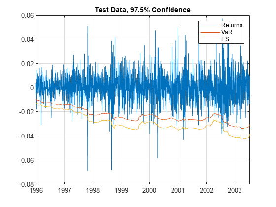
Use the plot function to visualize the ES backtesting data. This type of visualization is a common first step when performing an ES backtesting analysis. This plot displays the returns data against the VaR and ES data.
VaRInd = 2;
figure;
plot(Dates,Returns,Dates,-VaR(:,VaRInd),Dates,-ES(:,VaRInd))
legend('Returns','VaR','ES')
title(['Test Data, ' num2str(VaRLevel(VaRInd)*100) '% Confidence'])
grid on

Step 3. Create an esbacktestbysim object.
Create an esbacktestbysim object using esbacktestbysim. The Distribution information is used to simulate returns to estimate the significance of the tests. The simulation to estimate the significance is run by default when you create the esbacktestbysim object. Therefore, the test results are available when you create the object. You can set the optional name-value input argument Simulate to false to avoid the simulation, in which case you can use the simulate function before querying for test results.
rng('default'); % for reproducibility
IDs = ["t(dof) 95%","t(dof) 97.5%","t(dof) 99%"];
IDs = strrep(IDs,"dof",num2str(DoF));
ebts = esbacktestbysim(Returns,VaR,ES,Distribution,...
   'DegreesOfFreedom',DoF,...
   'Location',Mu,...
   'Scale',Sigma,...
   'PortfolioID',"S&P",...
   'VaRID',IDs,...
   'VaRLevel',VaRLevel);
disp(ebts)
  esbacktestbysim with properties:

    PortfolioData: [1966×1 double]
          VaRData: [1966×3 double]
           ESData: [1966×3 double]
     Distribution: [1×1 struct]
      PortfolioID: "S&P"
            VaRID: ["t(10) 95%"    "t(10) 97.5%"    "t(10) 99%"]
         VaRLevel: [0.9500 0.9750 0.9900]
disp(ebts.Distribution) % distribution information stored in the 'Distribution' property Name: "t"
DegreesOfFreedom: 10
Location: 0
Scale: [1966×1 double]
Step 4. Generate the ES summary report.
The ES summary report provides information about the severity of the violations, that is, how large the loss is compared to the VaR on days when the VaR was violated. The ObservedSeverity (or observed average severity ratio) column is the ratio of loss to VaR over days when the VaR is violated. The ExpectedSeverity (or expected average severity ratio) column shows the average of the ratio of ES to VaR on the days when the VaR is violated.
S = summary(ebts);
disp(S)
    PortfolioID        VaRID        VaRLevel    ObservedLevel    ExpectedSeverity    ObservedSeverity    Observations    Failures    Expected    Ratio     Missing
    ___________    _____________    ________    _____________    ________________    ________________    ____________    ________    ________    ______    _______

       "S&P"       "t(10) 95%"        0.95         0.94812            1.3288              1.4515             1966          102         98.3      1.0376       0
       "S&P"       "t(10) 97.5%"     0.975         0.97202            1.2652              1.4134             1966           55        49.15       1.119       0
       "S&P"       "t(10) 99%"        0.99         0.98627            1.2169              1.3947             1966           27        19.66      1.3733       0
Step 5. Run a report for all tests.
Run all tests and generate a report on only the accept or reject results.
t = runtests(ebts);
disp(t)
    PortfolioID        VaRID        VaRLevel    Conditional    Unconditional    Quantile    MinBiasAbsolute    MinBiasRelative
    ___________    _____________    ________    ___________    _____________    ________    _______________    _______________

       "S&P"       "t(10) 95%"        0.95        reject          accept         reject         accept             reject
       "S&P"       "t(10) 97.5%"     0.975        reject          reject         reject         reject             reject
       "S&P"       "t(10) 99%"        0.99        reject          reject         reject         reject             reject
Step 6. Run the conditional test.
Run the individual test for the conditional test (also known as the first Acerbi-Szekely test). The second output (s) contains simulated test statistic values, assuming the distributional assumptions are correct. Each row of the s output matches the VaRID in the corresponding row of the t output. Use these simulated statistics to determine the significance of the tests.
[t,s] = conditional(ebts);
disp(t)
    PortfolioID        VaRID        VaRLevel    Conditional    ConditionalOnly    PValue    TestStatistic    CriticalValue    VaRTest    VaRTestResult    VaRTestPValue    Observations    Scenarios    TestLevel
    ___________    _____________    ________    ___________    _______________    ______    _____________    _____________    _______    _____________    _____________    ____________    _________    _________

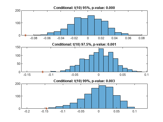
       "S&P"       "t(10) 95%"        0.95        reject           reject             0       -0.092302        -0.043941       "pof"        accept           0.70347           1966          1000         0.95
       "S&P"       "t(10) 97.5%"     0.975        reject           reject         0.001        -0.11714        -0.052575       "pof"        accept           0.40682           1966          1000         0.95
       "S&P"       "t(10) 99%"        0.99        reject           reject         0.003        -0.14608        -0.085433       "pof"        accept           0.11536           1966          1000         0.95
whos sName Size Bytes Class Attributes s 3x1000 24000 double
Step 7. Visualize the significance of the conditional test.
Visualize the significance of the conditional test using histograms to show the distribution of typical values (simulation results). In the histograms, the asterisk shows the value of the test statistic observed for the actual returns. This is a visualization of the standalone conditional test. The final conditional test result also depends on a preliminary VaR backtest, as shown in the conditional test output.
NumVaRs = height(t);
figure;
for VaRInd = 1:NumVaRs
   subplot(NumVaRs,1,VaRInd)
   histogram(s(VaRInd,:));
   hold on;
   plot(t.TestStatistic(VaRInd),0,'*');
   hold off;
   Title = sprintf('Conditional: %s, p-value: %4.3f',t.VaRID(VaRInd),t.PValue(VaRInd));
   title(Title)
end

Step 8. Run the unconditional test.
Run the individual test for the unconditional test (also known as the second Acerbi-Szekely test).
[t,s] = unconditional(ebts);
disp(t)
    PortfolioID        VaRID        VaRLevel    Unconditional    PValue    TestStatistic    CriticalValue    Observations    Scenarios    TestLevel
    ___________    _____________    ________    _____________    ______    _____________    _____________    ____________    _________    _________

       "S&P"       "t(10) 95%"        0.95         accept        0.093       -0.13342         -0.16252           1966          1000         0.95
       "S&P"       "t(10) 97.5%"     0.975         reject        0.031       -0.25011          -0.2268           1966          1000         0.95
       "S&P"       "t(10) 99%"        0.99         reject        0.008       -0.57396         -0.38264           1966          1000         0.95
Step 9. Visualize the significance of the unconditional test.
Visualize the significance of the unconditional test using histograms to show the distribution of typical values (simulation results). In the histograms, the asterisk shows the value of the test statistic observed for the actual returns.
NumVaRs = height(t);
figure;
for VaRInd = 1:NumVaRs
   subplot(NumVaRs,1,VaRInd)
   histogram(s(VaRInd,:));
   hold on;
   plot(t.TestStatistic(VaRInd),0,'*');
   hold off;
   Title = sprintf("Unconditional: %s, p-value: %4.3f",t.VaRID(VaRInd),t.PValue(VaRInd));
   title(Title)
end

Step 10. Run the quantile test.
Run the individual test for the quantile test (also known as the third Acerbi-Szekely test).
[t,s] = quantile(ebts);
disp(t)
    PortfolioID        VaRID        VaRLevel    Quantile    PValue    TestStatistic    CriticalValue    Observations    Scenarios    TestLevel
    ___________    _____________    ________    ________    ______    _____________    _____________    ____________    _________    _________

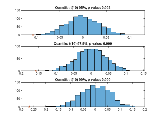
       "S&P"       "t(10) 95%"        0.95       reject     0.002       -0.10602         -0.055798          1966          1000         0.95
       "S&P"       "t(10) 97.5%"     0.975       reject         0       -0.15697         -0.073513          1966          1000         0.95
       "S&P"       "t(10) 99%"        0.99       reject         0       -0.26561          -0.10117          1966          1000         0.95
Step 11. Visualize the significance of the quantile test.
Visualize the significance of the quantile test using histograms to show the distribution of typical values (simulation results). In the histograms, the asterisk shows the value of the test statistic observed for the actual returns.
NumVaRs = height(t);
figure;
for VaRInd = 1:NumVaRs
   subplot(NumVaRs,1,VaRInd)
   histogram(s(VaRInd,:));
   hold on;
   plot(t.TestStatistic(VaRInd),0,'*');
   hold off;
   Title = sprintf("Quantile: %s, p-value: %4.3f",t.VaRID(VaRInd),t.PValue(VaRInd));
   title(Title)
end

Step 10. Run the minBiasAbsolute test.
Run the individual test for the minBiasAbsolute test.
[t,s] = minBiasAbsolute(ebts);
disp(t)
    PortfolioID        VaRID        VaRLevel    MinBiasAbsolute    PValue    TestStatistic    CriticalValue    Observations    Scenarios    TestLevel
    ___________    _____________    ________    _______________    ______    _____________    _____________    ____________    _________    _________

       "S&P"       "t(10) 95%"        0.95          accept         0.062      -0.0014247       -0.0015578          1966          1000         0.95
       "S&P"       "t(10) 97.5%"     0.975          reject         0.029      -0.0026674       -0.0023251          1966          1000         0.95
       "S&P"       "t(10) 99%"        0.99          reject         0.005      -0.0060982       -0.0039004          1966          1000         0.95
Step 11. Visualize the significance of the minBiasAbsolute test.
Visualize the significance of the minBiasAbsolute test using histograms to show the distribution of typical values (simulation results). In the histograms, the asterisk shows the value of the test statistic observed for the actual returns.
NumVaRs = height(t);
figure;
for VaRInd = 1:NumVaRs
   subplot(NumVaRs,1,VaRInd)
   histogram(s(VaRInd,:));
   hold on;
   plot(t.TestStatistic(VaRInd),0,'*');
   hold off;
   Title = sprintf('minBiasAbsolute: %s, p-value: %4.3f',t.VaRID(VaRInd),t.PValue(VaRInd));
   title(Title)
end

Step 10. Run the minBiasRelative test.
Run the individual test for the minBiasRelative test.
[t,s] = minBiasRelative(ebts);
disp(t)
    PortfolioID        VaRID        VaRLevel    MinBiasRelative    PValue    TestStatistic    CriticalValue    Observations    Scenarios    TestLevel
    ___________    _____________    ________    _______________    ______    _____________    _____________    ____________    _________    _________

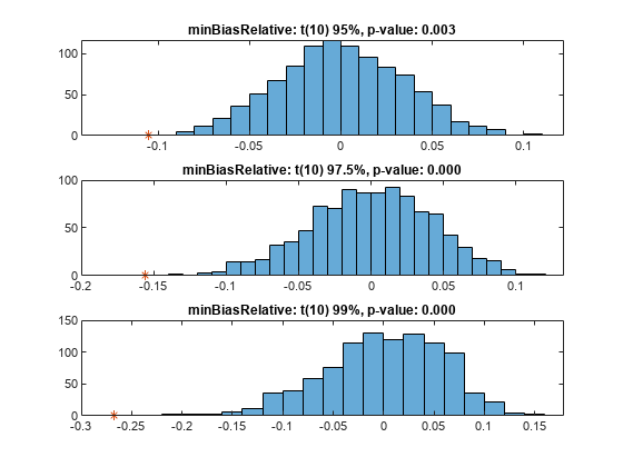
       "S&P"       "t(10) 95%"        0.95          reject         0.003       -0.10509         -0.056072          1966          1000         0.95
       "S&P"       "t(10) 97.5%"     0.975          reject             0       -0.15603         -0.073324          1966          1000         0.95
       "S&P"       "t(10) 99%"        0.99          reject             0       -0.26716            -0.104          1966          1000         0.95
Step 11. Visualize the significance of the minBiasAbsolute test.
Visualize the significance of the minBiasRelative test using histograms to show the distribution of typical values (simulation results). In the histograms, the asterisk shows the value of the test statistic observed for the actual returns.
NumVaRs = height(t);
figure;
for VaRInd = 1:NumVaRs
   subplot(NumVaRs,1,VaRInd)
   histogram(s(VaRInd,:));
   hold on;
   plot(t.TestStatistic(VaRInd),0,'*');
   hold off;
   Title = sprintf("minBiasRelative: %s, p-value: %4.3f",t.VaRID(VaRInd),t.PValue(VaRInd));
   title(Title)
end

Step 12. Run a new simulation to estimate the significance of the tests.
Run the simulation again using 5000 scenarios to generate a new set of test results. If the initial test results for one of the tests are borderline, using a larger simulation can help clarify the test results.
ebts = simulate(ebts,'NumScenarios',5000);
t = unconditional(ebts);  % new results for unconditional test
disp(t)
    PortfolioID        VaRID        VaRLevel    Unconditional    PValue    TestStatistic    CriticalValue    Observations    Scenarios    TestLevel
    ___________    _____________    ________    _____________    ______    _____________    _____________    ____________    _________    _________

       "S&P"       "t(10) 95%"        0.95         accept        0.0984      -0.13342         -0.17216           1966          5000         0.95
       "S&P"       "t(10) 97.5%"     0.975         reject        0.0456      -0.25011         -0.24251           1966          5000         0.95
       "S&P"       "t(10) 99%"        0.99         reject        0.0104      -0.57396         -0.40089           1966          5000         0.95
See Also
summary | runtests | conditional | unconditional | quantile | simulate | minBiasRelative | minBiasAbsolute