Control of a Spring-Mass-Damper System Using Mixed-Mu Synthesis

Open Script

This example shows how to perform mixed-mu synthesis with the musyn command in the Robust Control Toolbox™. Here musyn is used to design a robust controller for a two mass-spring-damper system with uncertainty in the spring stiffness connecting the two masses. This example is taken from the paper "Robust mixed-mu synthesis performance for mass-spring system with stiffness uncertainty," D. Barros, S. Fekri and M. Athans, 2005 Mediterranean Control Conference.

Performance Specifications

Consider the mass-spring-damper system in Figure 1. Spring k2 and damper b2 are attached to the wall and mass m2. Mass m2 is also attached to mass m1 through spring k1 and damper b1. Mass 2 is affected by the disturbance force f2. The system is controlled via force f1 acting on mass m1.

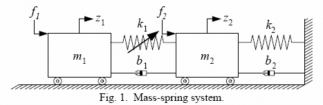
Our design goal is to use the control force f1 to attenuate the effect of the disturbance f2 on the position of mass m2. The force f1 does not directly act on mass m2, rather it acts through the spring stiffness k1. Hence any uncertainty in the spring stiffness k1 will make the control problem more difficult. The control problem is formulated as:

The controller measures the noisy displacement of mass m2 and applies the control force f1. The sensor noise, Wn, is modeled as a constant 0.001.

The actuator command is penalized by a factor 0.1 at low frequency and a factor 10 at high frequency with a crossover frequency of 100 rad/s (filter Wu).

The unit magnitude, first-order coloring filter, Wdist, on the disturbance has a pole at 0.25 rad/s.

The performance objective is to attenuate the disturbance on mass m2 by a factor of 80 below 0.1 rad/s.

The nominal values of the system parameters are m1=1, m2=2, k2=1, b1=0.05, b2=0.05, and k1=2.

Wn = tf(0.001);
Wu = 10*tf([1 10],[1 1000]);
Wdist = tf(0.25,[1 0.25],'inputname','dist','outputname','f2');
Wp = 80*tf(0.1,[1 0.1]);
m1 = 1;
m2 = 2;
k2 = 1;
b1 = 0.05;
b2 = 0.05;

Uncertainty Modeling

The value of spring stiffness k1 is uncertain. It has a nominal value of 2 and its value can vary between 1.2 and 2.8.

k1 = ureal('k1',2,'Range',[1.2 2.8]);

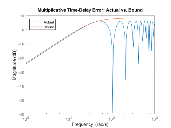
There is also a time delay tau between the commanded actuator force f1 and its application to mass m1. The maximum delay is 0.06 seconds. Neglecting this time delay introduces a multiplicative error of exp(-s*tau)-1. This error can be treated as unmodeled dynamics bounded in magnitude by the high-pass filter Wunmod = 2.6*s/(s + 40):

tau = ss(1,'InputDelay',0.06);
Wunmod = 2.6*tf([1 0],[1 40]);
bodemag(tau-1,Wunmod,logspace(0,3,200));
title('Multiplicative Time-Delay Error: Actual vs. Bound')
legend('Actual','Bound','Location','NorthWest')

Construct an uncertain state-space model of the plant with the control force f1 and disturbance f2 as inputs.

a1c = [0 0 -1/m1  1/m2]'*k1;
a2c = [0 0  1/m1 -1/m2]'*k1 + [0 0 0 -k2/m2]';
a3c = [1 0 -b1/m1 b1/m2]';
a4c = [0 1 b1/m1 -(b1+b2)/m2]';
A  = [a1c a2c a3c a4c];
plant = ss(A,[0 0;0 0;1/m1 0;0 1/m2],[0 1 0 0],[0 0]);
plant.StateName = {'z1';'z2';'z1dot';'z2dot'};
plant.OutputName = {'z2'};

Add the unmodeled delay dynamics at the first plant input.

Delta = ultidyn('Delta',[1 1]);
plant = plant * append(1+Delta*Wunmod,1);
plant.InputName = {'f1','f2'};

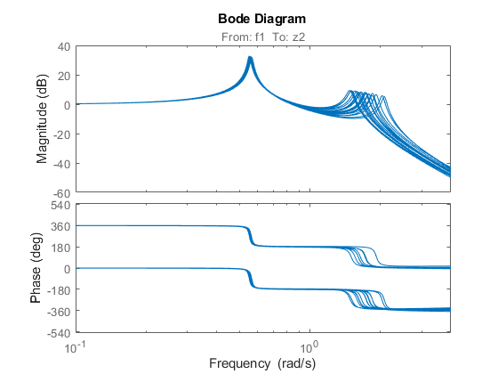
Plot the Bode response from f1 to z2 for 20 sample values of the uncertainty. The uncertainty on the value of k1 causes fluctuations in the natural frequencies of the plant modes.

bode(plant(1,1),{0.1,4})

Control Design

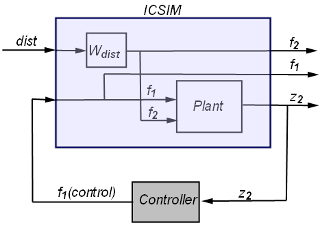
We use the following structure for controller synthesis:

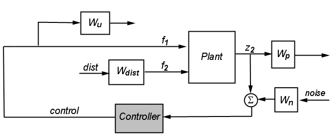
Figure 2

Use connect to construct the corresponding open-loop interconnection IC. Note that IC is an uncertain model with uncertain variables k1 and Delta.

Wu.u = 'f1';  Wu.y = 'Wu';
Wp.u = 'z2';  Wp.y = 'Wp';
Wn.u = 'noise';  Wn.y = 'Wn';
S = sumblk('z2n = z2 + Wn');
IC = connect(plant,Wdist,Wu,Wp,Wn,S,{'dist','noise','f1'},{'Wp','Wu','z2n'})

Uncertain continuous-time state-space model with 3 outputs, 3 inputs, 8 states.
The model uncertainty consists of the following blocks:
  Delta: Uncertain 1x1 LTI, peak gain = 1, 1 occurrences
  k1: Uncertain real, nominal = 2, range = [1.2,2.8], 1 occurrences

Type "IC.NominalValue" to see the nominal value and "IC.Uncertainty" to interact with the uncertain elements.

Complex mu-Synthesis

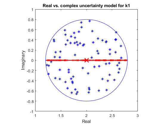
You can use the command musyn to synthesize a robust controller for the open-loop interconnection IC. By default, musyn treats all uncertain real parameters, in this example k1, as complex uncertainty. Recall that k1 is a real parameter with a nominal value of 2 and a range between 1.2 and 2.8. In complex mu-synthesis, it is replaced by a complex uncertain parameter varying in a disk centered at 2 and with radius 0.8. The plot below compares the range of k1 values when k1 is treated as real (red x) vs. complex (blue *).

k1c = ucomplex('k1c',2,'Radius',0.8);  % complex approximation

% Plot 80 samples of the real and complex parameters
k1samp = usample(k1,80);
k1csamp = usample(k1c,80);
plot(k1samp(:),0*k1samp(:),'rx',real(k1csamp(:)),imag(k1csamp(:)),'b*')
hold on

% Draw value ranges for real and complex k1
plot(k1.Nominal,0,'rx',[1.2 2.8],[0 0],'r-','MarkerSize',14,'LineWidth',2)
the=0:0.02*pi:2*pi;
z=sin(the)+sqrt(-1)*cos(the);
plot(real(0.8*z+2),imag(0.8*z),'b')
hold off

% Plot formatting
axis([1 3 -1 1]), axis square
ylabel('Imaginary'), xlabel('Real')
title('Real vs. complex uncertainty model for k1')

Synthesize a robust controller Kc using complex mu-synthesis (treating k1 as a complex parameter).

[Kc,mu_c,infoc] = musyn(IC,1,1);


D-K ITERATION SUMMARY:
-----------------------------------------------------------------
                       Robust performance               Fit order
-----------------------------------------------------------------
  Iter         K Step       Peak MU       D Fit             D
    1           2.954        2.452        2.483            16
    2           1.145        1.143        1.153            18
    3           1.086        1.086         1.09            18
    4           1.082        1.081        1.085            18
    5           1.085        1.084        1.087            18

Best achieved robust performance: 1.08

Note that mu_c exceeds 1 so the controller Kc fails to robustly achieve the desired performance level.

Mixed-Mu Synthesis

Mixed-mu synthesis accounts for uncertain real parameters directly in the synthesis process. Enable mixed-mu synthesis by setting the MixedMU option to 'on'.

opt = musynOptions('MixedMU','on');
[Km,mu_m] = musyn(IC,1,1,opt);


DG-K ITERATION SUMMARY:
-------------------------------------------------------------------
                       Robust performance                 Fit order
-------------------------------------------------------------------
  Iter         K Step       Peak MU       DG Fit           D      G
    1           2.954        2.081        2.367           16      8
    2           1.606        1.388        1.567           16     12
    3          0.9313        1.078        1.266           20      8
    4          0.9188       0.9789        1.093           20      8
    5          0.9111       0.9403       0.9797           20      8
    6          0.9075       0.9269        0.945           20      8
    7          0.9005       0.9126       0.9182           20      8
    8           0.892       0.9058       0.9262           20      8
    9          0.8945       0.9001       0.9209           18      8
   10          0.8928       0.8959       0.9109           18      8

Best achieved robust performance: 0.896

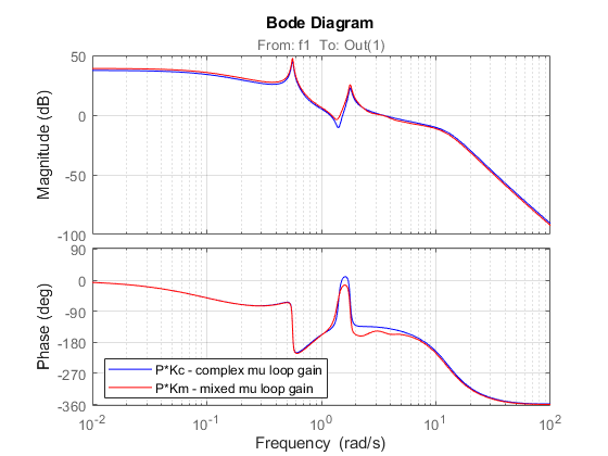
Mixed-mu synthesis is able to find a controller that achieves the desired performance and robustness objectives. A comparison of the open-loop responses shows that the mixed-mu controller Km gives less phase margin near 3 rad/s because it only needs to guard against real variations of k1.

clf
% Note: Negative sign because interconnection in Fig 2 uses positive feedback
bode(-Kc*plant.NominalValue(1,1),'b',-Km*plant.NominalValue(1,1),'r',{1e-2,1e2})
grid
legend('P*Kc - complex mu loop gain','P*Km - mixed mu loop gain','location','SouthWest')

Worst-Case Analysis

A comparison of the two controllers indicates that taking advantage of the "realness" of k1 results in a better performing, more robust controller.

To assess the worst-case closed-loop performance of Kc and Km, form the closed-loop interconnection of Figure 2 and use the command wcgain to determine how large the disturbance-to-error norm can get for the specified plant uncertainty.

clpKc = lft(IC,Kc);
clpKm = lft(IC,Km);
[maxgainKc,badpertKc] = wcgain(clpKc);
maxgainKc

maxgainKc = 

  struct with fields:

           LowerBound: 2.0817
           UpperBound: 2.0860
    CriticalFrequency: 1.4303

[maxgainKm,badpertKm] = wcgain(clpKm);
maxgainKm

maxgainKm = 

  struct with fields:

           LowerBound: 0.8906
           UpperBound: 0.8926
    CriticalFrequency: 0.1741

The mixed-mu controller Km has a worst-case gain of 0.88 while the complex-mu controller Kc has a worst-case gain of 2.2, or 2.5 times larger.

Disturbance Rejection Simulations

To compare the disturbance rejection performance of Kc and Km, first build closed-loop models of the transfer from input disturbance dist to f2, f1, and z2 (position of the mass m2).

Km.u = 'z2';  Km.y = 'f1';
clsimKm = connect(plant,Wdist,Km,'dist',{'f2','f1','z2'});
Kc.u = 'z2';  Kc.y = 'f1';
clsimKc = connect(plant,Wdist,Kc,'dist',{'f2','f1','z2'});

Inject white noise into the low-pass filter Wdist to simulate the input disturbance f2. The nominal closed-loop performance of the two designs is nearly identical.

t = 0:.01:100;
dist = randn(size(t));
yKc = lsim(clsimKc.Nominal,dist,t);
yKm = lsim(clsimKm.Nominal,dist,t);

% Plot
subplot(311)
plot(t,yKc(:,3),'b',t,yKm(:,3),'r')
title('Nominal Disturbance Rejection Response')
ylabel('z2')

subplot(312)
plot(t,yKc(:,2),'b',t,yKm(:,2),'r')
ylabel('f1 (control)')
legend('Kc','Km','Location','NorthWest')

subplot(313)
plot(t,yKc(:,1),'k')
ylabel('f2 (disturbance)')
xlabel('Time (sec)')

Next, compare the worst-case scenarios for Kc and Km by setting the plant uncertainty to the worst-case values computed with wcgain.

clsimKc_wc = usubs(clsimKc,badpertKc);
clsimKm_wc = usubs(clsimKm,badpertKm);
yKc_wc = lsim(clsimKc_wc,dist,t);
yKm_wc = lsim(clsimKm_wc,dist,t);

subplot(211)
plot(t,yKc_wc(:,3),'b',t,yKm_wc(:,3),'r')
title('Worse-Case Disturbance Rejection Response')
ylabel('z2')
subplot(212)
plot(t,yKc_wc(:,2),'b',t,yKm_wc(:,2),'r')
ylabel('f1 (control)')
legend('Kc','Km','Location','NorthWest')

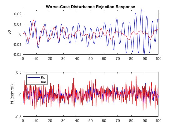
This shows that the mixed-mu controller Km significantly outperforms Kc in the worst-case scenario. By exploiting the fact that k1 is real, the mixed-mu controller is able to deliver better performance at equal robustness.

Controller Simplification

The mixed-mu controller Km has relatively high order compared to the plant. To obtain a simpler controller, use musyn's fixed-order tuning capability. This uses hinfstruct instead of hinfsyn for the synthesis step. You can try different orders to find the simplest controller that maintains robust performance. For example, try tuning a fifth-order controller. Use the "RandomStart" option to run several mu-synthesis cycles, each starting from a different initial value of K.

K = tunableSS('K',5,1,1);  % 5th-order tunable state-space model

opt = musynOptions('MixedMU','on','MaxIter',20,'RandomStart',2);
rng(0), [CL,mu_f] = musyn(lft(IC,K),opt);

=== Synthesis 1 of 3 ============================================


DG-K ITERATION SUMMARY:
-------------------------------------------------------------------
                       Robust performance                 Fit order
-------------------------------------------------------------------
  Iter         K Step       Peak MU       DG Fit           D      G
    1           22.12        15.05        15.21           10      6
    2           6.412        6.342        7.435           18      6
    3           6.473        6.402        6.472           18      6
    4           5.953        5.972        6.576           18      6
    5           6.011        5.946        6.871           20      6
    6           6.143        6.079        9.652           18      6

Best achieved robust performance: 5.95


=== Synthesis 2 of 3 ============================================


DG-K ITERATION SUMMARY:
-------------------------------------------------------------------
                       Robust performance                 Fit order
-------------------------------------------------------------------
  Iter         K Step       Peak MU       DG Fit           D      G
    1           3.368        3.258        3.259           16      8
    2           2.066         2.03         2.23           14      8
    3           1.567        1.566        2.736           16      8
    4           1.385        1.381        1.771           14      8
    5           1.213        1.213        1.531           18      8
    6           1.184        1.182         1.25           18      8
    7            1.12        1.119         1.24           20      8
    8           1.083        1.082        1.121           18      8
    9           1.052        1.052        1.175           20      8
   10           1.059        1.057        1.073           16      8
   11           1.035        1.034        1.162           18      8
   12           1.044        1.043        1.061           20      8
   13           1.025        1.024        1.114           20      8
   14           1.034        1.033        1.059           16      8
   15           1.027        1.026        1.087           16      8

Best achieved robust performance: 1.02


=== Synthesis 3 of 3 ============================================


DG-K ITERATION SUMMARY:
-------------------------------------------------------------------
                       Robust performance                 Fit order
-------------------------------------------------------------------
  Iter         K Step       Peak MU       DG Fit           D      G
    1           3.068        2.957        2.957           16      8
    2           1.983        1.939        1.951           18      8
    3           1.434        1.432        1.433           18      8
    4           1.149        1.147         1.42           20      8
    5           1.153        1.146        1.149           18      8
    6           1.032        1.065        1.398           18      8
    7           1.046        1.045        1.061           16      8
    8           1.019        1.018        1.135           18      8
    9           1.038        1.037        1.039           20      8
   10           1.016        1.015        1.135           18      8

Best achieved robust performance: 1.02

The best controller nearly delivers the desired robust performance (robust performance mu_f is close to 1). Compare the two controllers.

clf, bode(Km,getBlockValue(CL,'K'))
legend('Full order','5th order')