Real Mu Analysis
This example shows how to use Robust Control Toolbox™ to analyze the robustness of an uncertain system with only real parametric uncertainty. You compute the stability margins for a rigid body transport aircraft using an output feedback control law. For more information about the model, see "A Practical Approach to Robustness Analysis with Aeronautical Applications" by G. Ferreres. Stability analysis for systems with only real parametric uncertainty can cause numerical difficulties. In this example, you compare three methods for computing the stability margins for systems with only real parametric uncertainty.
Creating an Uncertain Model for a Transport Aircraft
The rigid body model of a large transport aircraft has four states, two inputs, and four outputs. The states are sideslip (beta), roll rate (p), yaw rate (r), and roll angle (phi). The inputs are rudder deflection (deltap) and aileron deflection (deltar). The outputs are lateral acceleration (ny), roll rate (p), yaw rate (r), and roll angle (phi). The state equations depend on 14 aerodynamic coefficients, each coefficient having 10 percent uncertainty.
Create the uncertainties for the aerodynamic coefficients.
deg2rad = pi/180;      % conversion factor from degs to radians
rad2deg = 1/deg2rad;   % conversion factor from radians to degs
gV = 0.146418;         % g/V
tan_theta0 = 0.14;     % tan(theta0)
alpha0 = 8*deg2rad;    % (rad)

Ybeta = ureal('Ybeta',-0.082,'Percentage',10);
Yp = ureal('Yp',0.010827,'Percentage',10);
Yr = ureal('Yr',0.060268,'Percentage',10);
Ydeltap = ureal('Ydeltap',0.002,'Percentage',10);
Ydeltar = ureal('Ydeltar',0.0118,'Percentage',10);
Lbeta = ureal('Lbeta',-0.84,'Percentage',10);
Lp = ureal('Lp',-0.76,'Percentage',10);
Lr = ureal('Lr',0.74,'Percentage',10);
Ldeltap = ureal('Ldeltap',0.095,'Percentage',10);
Ldeltar = ureal('Ldeltar',0.06,'Percentage',10);
Nbeta = ureal('Nbeta',0.092,'Percentage',10);
Np = ureal('Np',-0.23,'Percentage',10);
Nr = ureal('Nr',-0.114,'Percentage',10);
Ndeltar = ureal('Ndeltar',-0.151,'Percentage',10);
The state equations for the rigid body aircraft dynamics are:
A = [Ybeta (Yp+sin(alpha0)) (Yr-cos(alpha0)) gV; ...
    Lbeta  Lp Lr 0; Nbeta Np Nr 0; 0 1 tan_theta0 0];
B = [Ydeltap Ydeltar; Ldeltap Ldeltar; 0 Ndeltar; 0 0];
C = -1/gV*deg2rad*[Ybeta Yp Yr 0];
C = [C; zeros(3,1) eye(3)];
D = -1/gV*deg2rad*[Ydeltap Ydeltar];
D = [D; zeros(3,2)];
AIRCRAFT = ss(A,B,C,D);
The aircraft model has actuators for the rudder and the aileron. Each actuator is modeled using a second-order system and the resulting dynamics are added to the input of the rigid body model. P is the open-loop model of the aircraft and the actuators.
N1 = [-1.77, 399];
D1 = [1 48.2 399];
deltap_act = tf(N1,D1);

N2 = [2.6 -1185 27350];
D2 = [1 77.7 3331 27350];
deltar_act = tf(N2,D2);

P = AIRCRAFT*blkdiag(deltap_act,deltar_act);
Creating the Closed Loop System
A constant output feedback control law is used and the closed loop is created with the feedback command.
K = [-629.8858 11.5254 3.3110 9.4278; ...
  285.9496 0.3693 -2.6301 -0.5489];

CLOOP = feedback(P,K);
Stability Analysis: Power Iteration
You can use robstab to compute robust stability margins for this system. This example focuses on the methods to compute lower bounds on mu, which is equivalent to computing the upper bound on the stability margin. By default, robstab uses a combination of power iteration and gain-based lower bound to compute the mu lower bound. First examine power iteration. The 'm' option for mussv is used to force robstab to use power iteration only.
ropt = robOptions('Mussv','m5','VaryFrequency','on');
[SM1,WCU1,INFO1] = robstab(CLOOP,ropt);
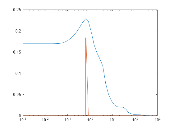
Power iteration is fast and typically provides good bounds for problems with complex uncertainty. However, it tends to perform poorly for systems with only real parametric uncertainty. For this example, power iteration finds a lower bound of zero for mu at most frequencies. Thus, the stability margin upper bound provides no information.
semilogx(INFO1.Frequency,1./INFO1.Bounds)
xlim([1e-3 1e3])

Figure 1: Mu bounds for Aircraft using power iteration lower bound.
Stability Analysis: Complexify the Real Uncertainty
One way to regularize this robust stability problem is to add a small amount of complex uncertainty to the real parametric uncertainty using the complexify command. Increasing alpha increases the complexity of the problem.
alpha = 0.05;
CLOOP_c = complexify(CLOOP,alpha);
There is a tradeoff when complexifying real uncertainty. Increasing the amount alpha of complex uncertainty improves the conditioning of the power iteration, thus increasing the chance of convergence. However, if you choose alpha too large, then you change the problem enough that the destabilizing perturbation for the modified problem may be far from destabilizing for the original problem.
[SM2,WC2,INFO2] = robstab(CLOOP_c,ropt);
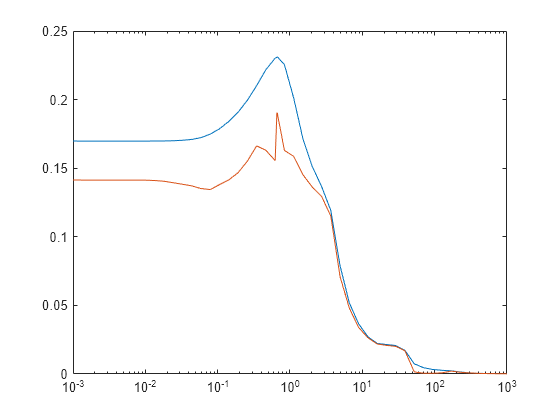
The plot shows the upper/lower mu bounds for the complexified problem. The upper bound is relatively unchanged by the complexification, and therefore complexification does not change the problem significantly.
semilogx(INFO2.Frequency,1./INFO2.Bounds)
xlim([1e-3 1e3])

Figure 2: Mu bounds for Aircraft using power iteration + complexify lower bound.
Stability Analysis: Gain-Based Lower Bound
For some problems, the amount of complexity necessary to regularize the lower bound significantly changes the problem and you should use the gain-based lower bound instead. Set 'g' as mussv option to force robstab to use the gain-based lower bound. Note that this approach is computationally slower compared to using power iteration and complexifying.
ropt = robOptions('Mussv','g','VaryFrequency','on');
[SM3,WC3,INFO3] = robstab(CLOOP,ropt);

semilogx(INFO3.Frequency,1./INFO3.Bounds)
xlim([1e-3 1e3])

Figure 3: Mu bounds for Aircraft using gain-based lower bound.