Globally Adapt Receiver Components in Time Domain

Receiver Component Global Adaptation Overview:

The receiver components for CTLE and DFECDR can work together to perform adaptation in Time Domain simulation. Normally, they operate independently as follows:

You can follow these steps to customize the CTLE and DFECDR to share signals within the RX system to adapt together globally during Time Domain simulation:

Part 1: Determine A Method for Optimizing RX Waveform vs. Equalization

You will see how equalization can affect RX waveforms to be either over-equalized, under-equalized, or critically-equalized (e.g. similar to how filter responses can be defined as over-damped, under-damped, or critically-damped).

Note: The concept of data words (3 symbols per word) from Communications Theory is used in this example.

Low Frequency (LF) and a High Frequency (HF) data word are defined for this example as follows:

Note: a CTLE block optimizes for inner-eye (HF content only).

Part 2: Customize Simulink Blocks in Receiver Section

Part 3: Implement Custom MATLAB Function to Adapt Equalization during Time Domain Simulation

Note: Blocks within the RX system can share signals. This is also true within the TX system. However, no signals can be shared between RX and TX systems.

Part 1: Determine a Method for Optimizing Receiver Waveform vs. Equalization

Initialize SerDes System with CTLE and DFECDR in the Receiver

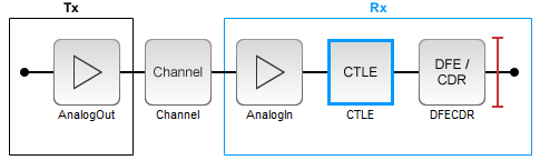
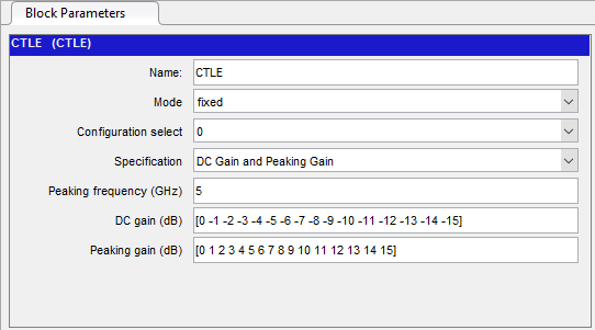
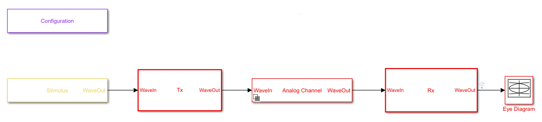
Open the system by typing serdesDesigner(‘TDadapt.mat’). You will see a system with a basic TX, 100-ohm channel with a loss of 16dB at 5GHz, and an RX containing a CTLE followed by a DFECDR. In this example, the CTLE is customized to use "fixed" mode (because this example shows how to programatically adapt by evaluating fixed values in a MATLAB function), and specification set to "DC Gain and Peaking Gain," and set "DC gain" to a range of 0 to -15 dB (in increments of -1dB), and set "Peaking gain" to a range of 0 to +15dB (in increments of +1dB) as shown below. Also note that the DFECDR should be set to "adapt" mode.

You can click on the CTLE and set the mode to "fixed."

Then you can cycle through different values for Configuration Select for the CTLE and observe the effect of different equalization values on the receiver eye diagram:

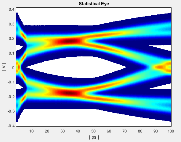
Figure Above: Under-equalized RX waveform: CTLE Configuration Select set to 0 (minimum).

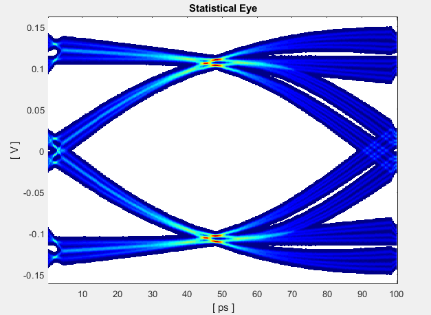
Figure Above: Over-equalized RX waveform: CTLE Configuration Select set to 15 (maximum).

Figure Above: Critically-equalized signal: CTLE Configuration Select set to 7 (e.g. a midrange value).

You can develop an algorithm to optimize the receiver signal by using the concept of Equalization. For example, an RX signal can be considered as being over-equalized, under-equalized, or critically-equalized:

Part 2: Customize Simulink Blocks in Receiver System

Export the system to Simulink.

Inside the Receiver section, you can modify the CTLE and DFECDR to share values using Signals in order to enable global adaptation during Time Domain simulation.

Modify the CTLE

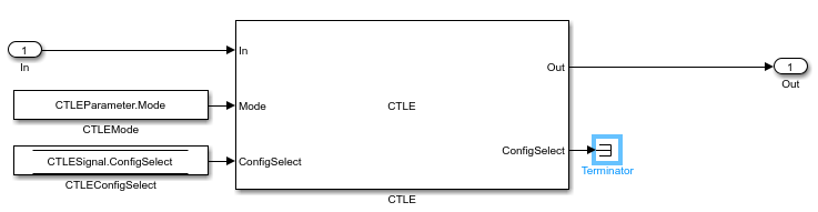
You can look under the CTLE mask (CTRL-U), then change the ConfigSelect output to a Terminator instead of a DataStoreWrite. By placing a Terminator at the ConfigSelect output, the CTLE is no longer in feedback mode, and any other block in the RX system can take control of this CTLE by writing to its ConfigSelect input signal.

You can click on the canvas and type "terminator" to create one, and then change the CTLE.ConfigSelect output to connect to a terminator as shown below:

Add CTLE Adaptation to the DFECDR

You can now modify the DFECDR to control the value of ConfigSelect input used by the CTLE during Time Domain simulation. This can be accomplished by adding a MATLAB function that uses the following parameters to evaluate a CTLE configuration to adapt to the next best equalization value:

• Mode

• ConfigIn

• symbolRecovered

• voltageSample

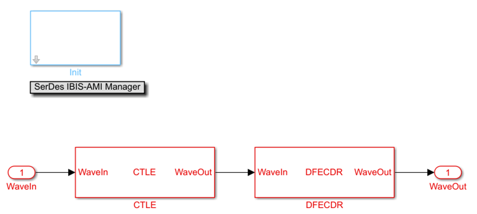
Next, you will see how to change the DFECDR to add this MATLAB function. From the Rx canvas, click on the DFECDR block and look under the mask (CTRL-U) to see the following:

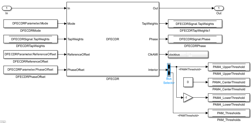
You will see a bus selector at the output port Interior. Double click to open its Block Parameters menu as shown:

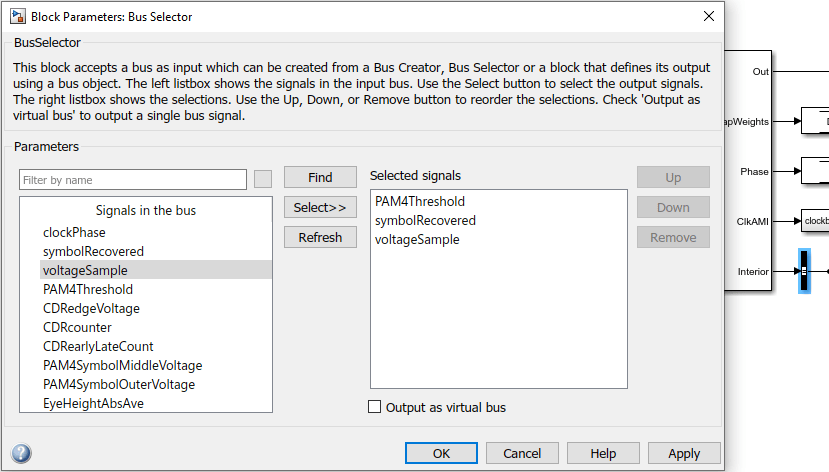
Click on signal symbolRecovered and click button "Add to output" and repeat this for voltageSample so the Output elements now include the following:

As shown below:

These elements are optional outputs, which is why you have to take steps enable them.

Create MATLAB Function to Enable CTLE Adaptation in Time Domain

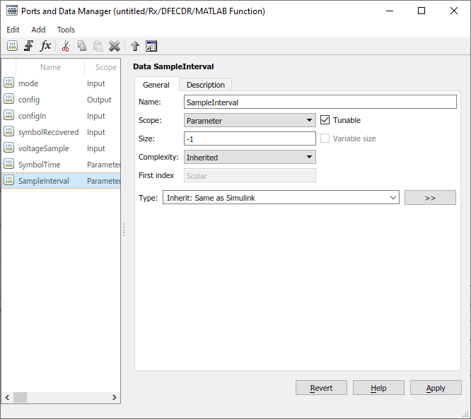
Next, add a MATLAB function to the Simulink canvas. You can get Simulink to automatically generate the ports by defining the function statement line of code as follows:

%  ctleTimeDomainAdapt - Simple adaptation algorithm to optimize a CTLE configuration
%                        in the time domain for NRZ signals.  Current serdes.CTLE
%                        adapts in Init/Statistical only.
%
%  Goal is to monitor the symbol decisions and voltage level of decisions from the
%  serdes.DFECDR.  From this, calculate the high and low frequency voltage averages to 
%  adjust the CTLE config bringing the averages together. Once settled, detect toggle
%  of config and lock adapted configuration.  The config adjustment operates under the
%  assumption that the CTLE 'boost' increases with increasing config from 0 to X and
%  modulation is NRZ only.

%   Copyright 2020 The MathWorks, Inc.

function config = ctleTimeDomainAdapt(mode, configIn, symbolRecovered, voltageSample, SampleInterval, SymbolTime)

Note: You can either use the code snippets concatenated as they are explained in this example, or you can use the attached MATLAB function "ctleTimeDomainAdapt.m" for reference.

Alternatively you can use the canvas tools in Simulink to create the ports. Using either method, the ports should appear as follows:

Inputs:

Output (same as function name):

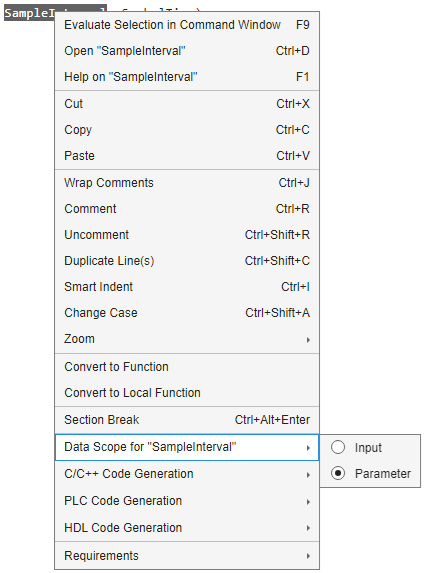
While in the function editor, change the Data Scope of symbolTime and sampleInterval from "signal" to "parameter" by right-clicking on the arguments in the function call:

Incorporate MATLAB function into Model

You will see how to incorporate this new function into the model in the following steps:

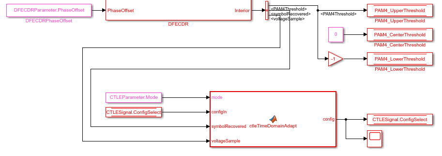
Note: you can add a Scope to observe the adapting values of CTLESignal.ConfigSelect during simulation.

When you are finished connecting the signals, the DFECDR will appear as follows:

Part 3: Implement Algorithm to Adapt Equalization during Time Domain Simulation

You can edit the file "ctleTimeDomainAdapt.m" attached to this example as a starting point for your adaptation algorithm. This example makes use of Persistent variables to keep track of values each time the MATLAB function is called. As a starting point, you will evaluate if the variables are non-zero (e.g. using function isempty()), so that when the first time the function is called, they can be initialized. After this point, their values will be configured by the CTLE and DFECDR blocks working together.

    persistent sps sampleCounter symbolCounter
    persistent internalConfig updateConfig symbols voltages 
    persistent lowFreqCount highFreqCount lowFreqVoltage highFreqVoltage
    persistent preventToggle toggling

    if isempty(sps)
        sps = SymbolTime/SampleInterval;
        sampleCounter = 0; % Total samples
        symbolCounter = 0; % Total symbols
        internalConfig = configIn; % Take config from Init and set for initial config
%         internalConfig = 0;  % Use this instead to ignore value from Init
        updateConfig = false;
        symbols = [0 0 0]; % Symbol history (3)
        voltages = [0 0 0]; % Voltage at each symbol (3)
        lowFreqCount = 0; % Low frequency event count
        highFreqCount = 0; % High frequency event count
        lowFreqVoltage = 0; % Voltage sum at low frequency events
        highFreqVoltage = 0; % Voltage sum at high frequency events
        preventToggle = [0 0 0 0]; % Toggle tracker; last 4 config updates -1/+1
        toggling = false; % Toggle detected flag
    end  

Note: When a variable is Persistent, that variable retains its value. Otherwise they are instantiated as undefined for each time a MATLAB function is called.

Implement Watchdogs such as a Toggle Detector

You can implement many types of watchdog testing, but this example implements a toggle detector. If the CTLE is at a given value and begins to increment or decrement by 1 (e.g. 4-5, 5-4, 4-5) from word to word, the program will test for a toggle condition by detecting 3 repetitions. If true, it exits the loop, thus the CTLE retains its trained optimal value.

Note: You can see an example implementation of such an algorithm in the attached file.

    if mode == 2 && ~toggling

Understanding Data Slicers

You can use the signals symbolRecovered and voltageSample to process the RX waveform. But first, it is important to understand Data Slicer operation:

1. Each time the clock time occurs at the start of a UI,

2. The DFECDR block applies its taps,

3. The data slicer is triggered at +0.5 UI later,

4. Then the tap value decision occurs for that bit.

A data slicer outputs both a symbol and a voltage. For example, if the data slicer operates at the 0.5 UI location, the slicer outputs a symbol as +0.5 or -0.5 and voltage value the symbol has reached.

Find UI Boundaries from Data Slicer

The system runs on a sample-based time step, so you can keep track of UI boundaries by setting up a sample and symbol counter. When a sample count is divisible by this setting for "samples per bit," this defines a symbol boundary. This way, you can find combinations of HF (e.g. 010, 101) or LF (e.g. 111, 000) data words to optimize for critical equalization:

       
        % How often to update CTLE Config
        updateFrequencySymbols = 1000;
        % Range of CTLE configurations
        minCTLEConfig = 0;
        maxCTLEConfig = 15;
        % Set up a sample and symbol counter to track overall progress
        sampleCounter = sampleCounter+1; % Every call to this function is a sample
        % When sample count is divisible by samples per bit, there is a symbol boundary
        if mod(sampleCounter,sps) == 0
            symbolCounter = symbolCounter+1;
            updateConfig = true; % Flag to keep from looping in update section 
            % Maintain bit/voltage history
            symbols = [symbols(2:3) symbolRecovered]; % -0.5 or 0.5
            voltages = [voltages(2:3) voltageSample]; % Voltages at each symbol
            % Keep count of low/high frequency events and sum voltages across those events
            % Low frequency = Steady high or low
            % High frequency = Rapid tranition
            if isequal(symbols, [0.5 0.5 0.5]) || isequal(symbols, [-0.5 -0.5 -0.5]) % 1 1 1 OR 0 0 0
                lowFreqCount = lowFreqCount + 1;
                lowFreqVoltage = lowFreqVoltage+ abs(voltages(2)); % keep middle voltage sample
            elseif isequal(symbols, [-0.5 0.5 -0.5]) || isequal(symbols, [0.5 -0.5 0.5])% 0 1 0 OR 1 0 1
                highFreqCount = highFreqCount + 1;
                highFreqVoltage = highFreqVoltage+ abs(voltages(2)); % keep middle voltage sample
            end
        end

Find 3-Symbol Combinations to Sort HF vs. LF Signal Content

You can use MATLAB function Mod to find when the samples/s has reached Mod 0, which defines the UI boundary. Once the symbol counter has reached modulo 0, you can accumulate these locations as bits. Then after accumulating sufficient bits (e.g. 1000), calculate the average of the voltages across this population, and update the CTLE Configuration.

Create an if statement to perform the following test and decision:

        % When symbol count is divisible by update frequency, check if CTLE update is needed
        if mod(symbolCounter,updateFrequencySymbols) == 0  && updateConfig
            % Calculate low/high voltage average
            lowFreqAvg = lowFreqVoltage/lowFreqCount;
            highFreqAvg = highFreqVoltage/highFreqCount;   

Update the CTLE

You can implement any algorithm you wish, but in this example the CTLE begins with configSelect value from Init, and the function performs an increment. Each time the DFECDR is evaluated and compared to a Persistent variable. Depending on this results, the CTLE is incremented or decremented.

Note: For the purposes of this function, be sure that CTLE is set to Mode = Fixed, and also only use valid values for configSelect in your model.

            % Increase CTLE config if low freq is above high freq
            if lowFreqAvg > highFreqAvg
                % Prevent exceeding maximum CTLE config
                if internalConfig < maxCTLEConfig
                    % If toggle is detected, disable adaptation
                    if ~isequal(preventToggle,[1 -1 1 -1])
                        internalConfig = internalConfig + 1;
                        % Add current action to toggle tracker
                        preventToggle = [preventToggle(2:4) 1];
                    else
                        toggling = true;
                    end
                end
            % Decrease CTLE config if high freq is above low freq
            elseif lowFreqAvg <= highFreqAvg
                % Prevent exceeding minimum CTLE config
                if internalConfig > minCTLEConfig
                    if ~isequal(preventToggle,[-1 1 -1 1])
                        internalConfig = internalConfig - 1;
                        % Add current action to toggle tracker
                        preventToggle = [preventToggle(2:4) -1];
                    else
                        toggling = true;
                    end
                end
            end
            % Reset variables associated with averaging every updateFrequencySymbols
            lowFreqCount = 0;
            lowFreqVoltage = 0;
            highFreqCount = 0;
            highFreqVoltage = 0;
            updateConfig = false; % Lock updates until next symbol boundary
        end
    end
    
    config = internalConfig;
end

Figure: Eye Diagram during Time Domain simulation.

You can see on the Scope that the CTLE started with the value from Init, and the toggle-detector code "locks" the CTLE configuration after a few iterations:

Figure: When Time Domain simulation begins, the CTLE starts with the value from Init.

You can set the code to start from CTLE configuration 0 and see that the algorithm increments the configuration until it toggles:

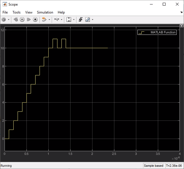
Figure: Scope output from the signal CTLESignal.ConfigSelect if the function is programmed to start from zero instead of the value from Init.

To find the value for Ignore Bits for the receiver, you can evaluate how many UI it takes for a CTLE to settle. In this case, it would be equal to the number of CTLE configurations available.

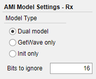
Figure: You can set the value for Ignore Bits to 16, which is the number of CTLE configurations available in this example.

When the simulation completes, you can see the Time Domain Eye has a valid Bathtub Curve if the simulation uses sufficient Ignore Bits for the receiver.

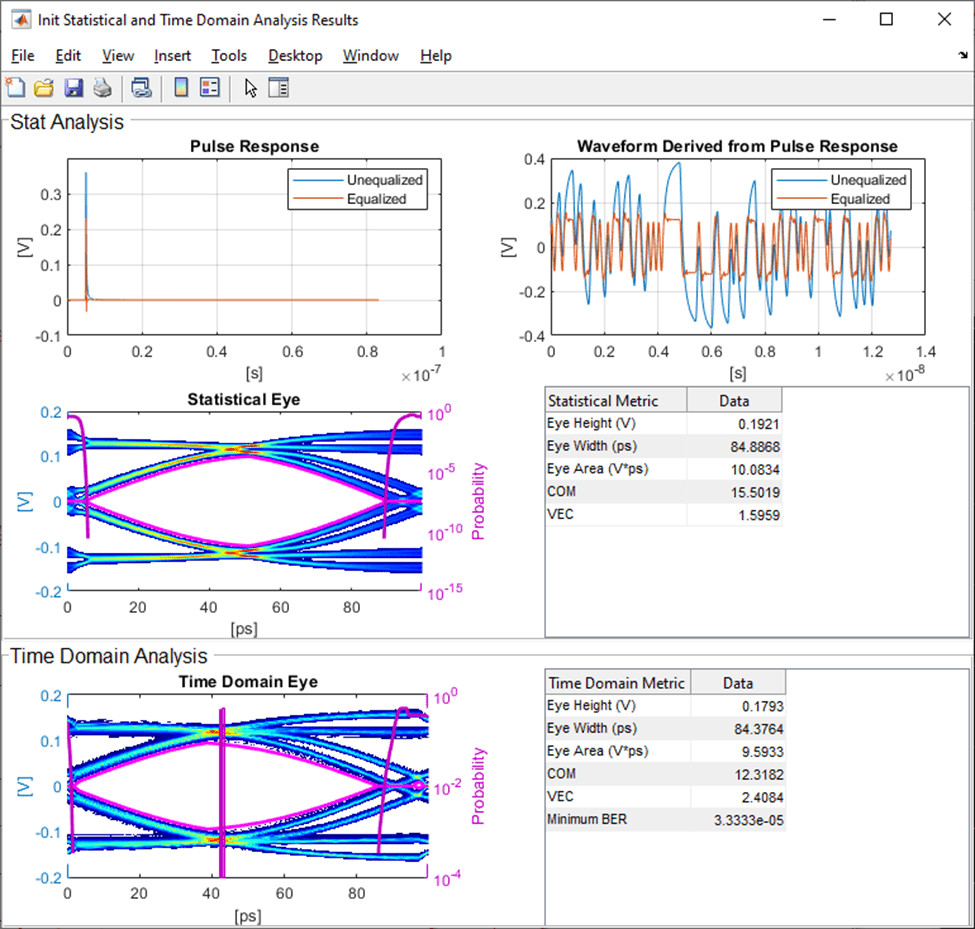
Figure: Statistical and Time Domain Results with sufficient Ignore Bits.

You can test the effect of Ignore Bits by setting the value to zero and re-running the simulation:

Figure: You can set the value for Ignore Bits to 0 from 16 to test its effect of Time Domain results.

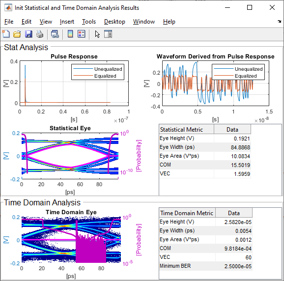
Figure: Statistical and Time Domain Results with insufficient Ignore Bits.