Explore Signal Integrity Interface with Design of Experiments and Response Surface Modeling

This example uses:

This example shows how to setup and create a Design of Experiments (DOE) using the MATLAB® scripting interface in the Signal Integrity Toolbox™. You can simulate dozens of cases and use the Statistical and Machine Learning Toolbox™ to fit and analyze a linear model.

Exploring a solution space with a large number of variables, each with multiple possible values, requires a lot of computation resources and time. It is not typically feasible to exhaustively simulate every factor combination. Alternatively, when you are searching for the best- or worst-case factor conditions, sweeping one variable at a time can lead to sub-optimal optimization due to local maximums and minimums. A well-established methodology, DOE and Response Surface Modeling (RSM), is a powerful way to sample the solution space and fit a polynomial model to the data. You can use the resulting model to predict the best- or worst-case conditions or leverage it as a surrogate model for advanced analysis.

To learn more about design of experiments, see Design of Experiments (Statistics and Machine Learning Toolbox). To learn how to use the Serial Link Designer app, see Analyze Backplane with Line Cards.

Open Signal Integrity Toolbox Project

For this experiment, use a 3-inch differential stripline transmission line (Tline). Configure the stripline properties of dielectric height, trace width, trace thickness, and dielectric constant to obtain the best system performance. The compressed folder DOETLine.zip attached with this example contains a Serial Link Designer project DOETLine. The project is already configured so it allows you to vary these solution space variables.

Serial Link Designer projects have several levels of folders. On Windows® operating systems the resulting path length can exceed the maximal character requirements and can result in confusing error messages. Therefore, for Windows operating systems, create the directory C:\SLD and copy the example files there. Unzip the file DOETLine.zip and open the file DOETlineExampleRunMe.mlx to run the example.

%Open Signal Integrity Project
sip = SignalIntegrityProject('DOETLine',opendesigner=true);
%Put in non-case mode (permutation mode)
sip.Interfaces(1).Sheets(1).CaseMode = false;

Get Solution Space Variables with Multiple Values

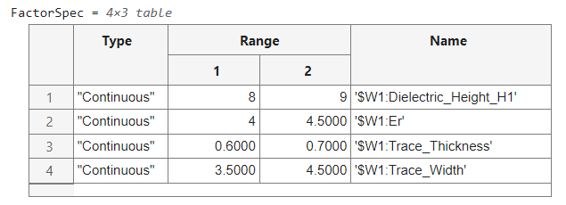
In this example, DOE factors are defined by setting the solution space variables to more than one value in the non-case mode (permutation mode) solution space. For each of the variables Dielectric_Height_H1, Er, Trace_Thickness, and Trace_Width, three value columns are defined. The code below searches the solution space and identifies the varying factors, their ranges, and variable type.

%Get Solution Space
SolutionSpaceTable = sip.Sheets(1).SolutionSpace.Table;

%Variable names
variableNames = SolutionSpaceTable.Properties.VariableNames;

%Find Value columns that start with Value_
valueColumnsIndex = ~cellfun(@isempty,regexp(variableNames,'^Value_'));

%Figure out which Value columns have multiple values
valueColumns = SolutionSpaceTable(:,valueColumnsIndex);
rowsWithMoreThanOneValue = sum(~ismissing(valueColumns),2)>1;

%Define DOE variable as Solution Space variables with more than one value
%column.
doeVariables = SolutionSpaceTable(rowsWithMoreThanOneValue,:);
doeVariablesArray = doeVariables.Variables;
doeVariablesArrayValues = doeVariablesArray(:,valueColumnsIndex);

NumberOfVariables = height(doeVariables);

%Define Factor specification for DOE
FactorSpec = cell(NumberOfVariables,3);
unitStr = cell(NumberOfVariables,1);
for ii = 1:NumberOfVariables

    %Variable Name
    FactorSpec{ii,3} = doeVariables.Variable{ii};

    if strcmpi('Soft Range',doeVariables.Format(ii))
        FactorSpec{ii,1} = "Continuous"; %Variable Type
        
        %Get set of possible values
        variableSet = unique(doeVariablesArrayValues(ii,:));
        variableSet(ismissing(variableSet)) = [];

        %Determine unit
        unitStr{ii} = regexp(variableSet(1),'(mil|in)','match','once');

        %Strip out unit string
        vs2 = regexprep(variableSet,'(mil|in)$','');
        vs3 = str2double(vs2);

        %Define Variable range
        if isnan(vs3(1))
            tmp = sprintf('"%s" ',vs2);
            error('%s unable to be converted to double.',tmp)
            %If this happens, perhaps the above unit search and replace
            %needs to be expanded to include new units.
        else
            FactorSpec{ii,2} = [min(vs3),max(vs3)]; %Variable Range
        end

    elseif strcmpi('List',doeVariables.Format(ii))
        %Get set of possible values
        variableSet = unique(doeVariablesArrayValues(ii,:));
        variableSet(ismissing(variableSet)) = [];

        if isnan(str2double(variableSet{1}))
            FactorSpec{ii,1} = "Categorical"; %Variable Type
            FactorSpec{ii,2} = cellstr(variableSet); %Variable Range
        else
            FactorSpec{ii,1} = "Discrete Numeric"; %Variable Type
            variableSet = str2double(variableSet);
            FactorSpec{ii,2} = variableSet; %Variable Range           
        end

    else
        error('Solution Space Format %s Unknown.',doeVariables.Format(ii))
    end

end

%Create Factor Specification table
FactorSpec = cell2table(FactorSpec, "VariableNames", ...
    ["Type", "Range", "Name"])

Continuous factors represent variables that can take any numeric value within its range. Categorical factors are used for string like variables like Corner which can have values of SS, TT, or FF. Discrete Numeric factors are for numerical variables that can only take certain values likes integers such as 0, 1, 2, 3, and more.

When applying this methodology to your own project, set up the Serial Link Designer app with the settings and options you want to use. Set the variables to more than one values to identify them as DOE factors. If your project uses Variation Groups, you need to modify the script to ensure that these connected variables vary together.

Create Design

After identifying the factors, use design of experiments to sample the solution space to increase the chances of obtaining a good model fit for a quadratic model, including terms for the constant, linear, interaction, and squared terms.

%Determine the number of runs
if iscell(FactorSpec.Range)
    nruns = sum(cellfun(@numel, FactorSpec.Range)) + 30;
else
    n = height(FactorSpec);
    nruns = 2^n + 20;
end

ntries = 5;
model = 'quadratic'; %Quadratic: Constant, linear, interaction and squared terms
DOEFactorCaseValues = makedesign(FactorSpec,nruns,'NumTries',ntries,'Model',model)

Write DOE Factor Cases to Solution Space

After identifying the DOE factor values, update the Serial Link Designer app solution space.

%Enable Case Mode
sip.Interfaces(1).Sheets(1).CaseMode = true;

%Reset Case Mode so there is only one case.  Use the first column in
%non-case mode (permutation mode) as the default. 
varNames = SolutionSpaceTable.Variable;
for ii = 1:length(varNames)
    sip.Interfaces(1).Sheets(1).SolutionSpace.updateSolutionSpace(...
        varNames(ii),SolutionSpaceTable.Value_1(ii));
end

%Set Design Of Experiments variable values
for ii = 1:width(DOEFactorCaseValues)
    
    %Define unit
    if isempty(unitStr{ii}) || any(ismissing(unitStr{ii}))
        varUnit = '';
    else        
        varUnit = unitStr{ii};
    end
    
    %Determine case value string
    if isempty(varUnit)
        caseValues = string(DOEFactorCaseValues{:,ii});
    else
        caseValues = strings(1,height(DOEFactorCaseValues));
        for jj = 1:nruns
            caseValues(jj) = sprintf('%s%s',string(DOEFactorCaseValues{jj,ii}),varUnit);
        end
    end

    %Update Solution Space for each DOE Factor
    sip.Interfaces(1).Sheets(1).SolutionSpace.updateSolutionSpace(...
        string(FactorSpec.Name{ii}),caseValues);
end

Run Simulations

Run the simulations.

%Ensure parallel simulations are used
sip.Parallel = true;

%Ensure Time Domain Analysis is off and Statistical Analysis is on
sip.simulationSetup("includeStatisticalAnalysis",true,"includeTimeDomainAnalysis",false);

%Run!
sip.run

Statistical Simulation Results

When the simulations complete, gather the results. Use the statistical eye height at a BER of 1e-12 as the system performance metric. Combine this with the DOE factor values and fit a linear quadratic model to the data. When fitting any model to data, be wary of and avoid over-fitting. Always look for the simplest model that explains the data adequately.

%Get statistical simulation results
ResultsTable = sip.Interfaces(1).Sheets(1).Results;

%Get Eye height data
hdr = ResultsTable.Properties.VariableNames';
ehColumn = find(strcmp(hdr,'Stat Eye Height[1e-12] (V)'));
eh = ResultsTable(:,ehColumn);

%Combine DOE Factors values with system response (eye height)
tableForFitting = [DOEFactorCaseValues,eh];

%Fit linear model.  Ideally use the same model for fitting as used in the
%DOE case determination above.
lm = fitlm(tableForFitting,'quadratic');

Visualize Fit

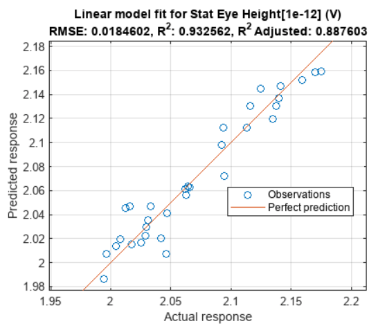
The Actual vs. Predicted plot is a great summary of the fit performance. A perfect fit will result in all observation cases laying on the perfect line. R-squared is a metric that measures the variation within a regression model and is ideally 1 and at worst 0. R-squared adjusted is a modified R-squared metric which penalizes for including irrelevant predictors in the model.

%Create Actual vs Predicted plot
ypred = predict(lm,DOEFactorCaseValues); %Predicted response
actual = eh{1:end,1};   %Actual response

%Determine range of perfect predition line
minv = min([ypred;actual]);
maxv = max([ypred;actual]);
perfect = [minv,maxv]+(maxv-minv)*0.05*[-1 1];

%Visualize
plot(actual,ypred,'o',perfect,perfect),
grid on
axis equal
legend('Observations','Perfect prediction','location','best')
xlabel('Actual response')
ylabel('Predicted response')
title(sprintf('Linear model fit for %s\nRMSE: %g, R^2: %g, R^2 Adjusted: %g',...
    lm.ResponseName,lm.RMSE,lm.Rsquared.Ordinary,lm.Rsquared.Adjusted))

An R-squared value of 0.95 and R-squared adjusted of 0.90 or greater is typically an indication of a good fit for signal integrity simulation model fits. This fit could be improved by eliminating uncontrolled parameters (such as the adaptive CTLE and the adaptive DFE) or by decreasing the range of each factor.

Visualize Residuals

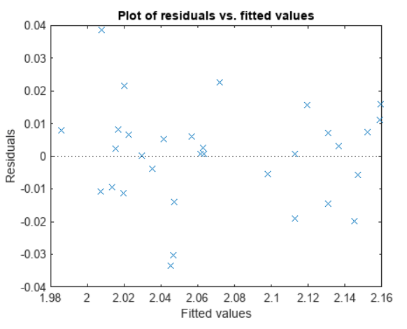
A residual is the difference between the actual and predicted performance. A residual plot that contains some structure and is not randomly distributed is an indication that more predictors could be used to improve the model fit. The residual plot below appears random and does not contain exploitable structure.

plotResiduals(lm,'fitted');

View Prediction Slice Plots

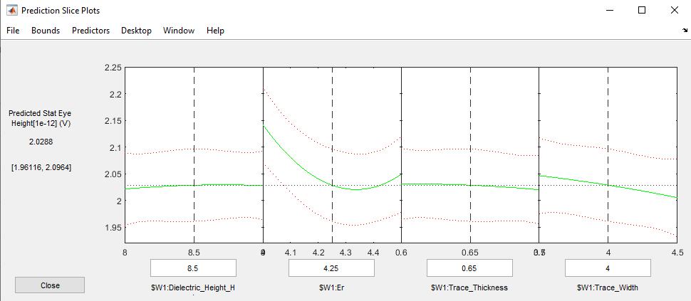
Use the prediction slice plot to visualize the profile of a multi-dimensional continuous model. Click and drag the vertical dashed line for each factor to explore the factor space and find the combination of factors that maximize system performance. For this fit, minimizing the dielectric constant Er, minimizing the trace width, maximizing the dielectric height H1 and setting the trace thickness to 0.64 results in the predicted maximum system performance.

plotSlice(lm)

Close Signal Integrity Project

sip.exit

Next Steps

Explore further by modifying the factor ranges, by adding other factors to the fit, and by using other fit models. The Regression Learner app in the Statistics and Machine Learning Toolbox is a very powerful in its ability to explore the effectiveness of a large variety of models.

Additionally, take the predicted best- and worst-case factor values and simulate them to double check that the actual predicted value is contained within the error bars of the fit.

References

How Design of Experiments Saved my CEI VSR 28G Design | 2016-09-18 | Signal Integrity Journal

Helper Functions

function t1 = makedesign(FactorSpec,NumRuns,NVArgs)
%Function to make a design from a specification table

arguments
    FactorSpec
    NumRuns
    NVArgs.NumTries {mustBePositive,mustBeInteger} = 1
    NVArgs.Model = 'linear'
end

nfactors = height(FactorSpec);
[bounds,iscat] = makebounds(FactorSpec,NVArgs.Model);
d1 = rowexch(nfactors, NumRuns, NVArgs.Model, "Bounds",bounds, "Tries",NVArgs.NumTries, "Categorical",iscat);
t1 = array2table(d1,"VariableNames",FactorSpec.Name);
t1 = applylevels(t1,FactorSpec);
end


function [bnds,iscat] = makebounds(spec,model)
% Function to make the 'bounds' input from the specification table

nfactors = height(spec);
range = spec.Range;
type = spec.Type;
if isnumeric(range)
    bnds = cell(size(range,1),1);
    for ii = 1:size(range,1)
        bnds{ii} = range(ii,:);
    end
    range = bnds;
else
    bnds = range;
end
iscat = false(1,nfactors);
for j = 1:nfactors
    switch(type{j})
        case "Continuous"
            % do error checking
            if model=="linear"
                bnds{j} = 0:1;
            else
                bnds{j} = [0 .5 1];
            end
        case "Discrete Numeric"
            % use group numbers, fix up later
            bnds{j} = 1:numel(range{j});
        case "Categorical"
            % use group numbers, fix up later
            bnds{j} = 1:numel(range{j});
            iscat(j) = true;
    end
end
iscat = find(iscat);
end

function t = applylevels(t,spec)
%Function to convert standard values to the specified ranges or sets for each factor
nfactors = height(spec);
if isnumeric(spec.Range)
    range = cell(size(spec.Range,1),1);
    for ii = 1:size(spec.Range,1)
        range{ii} = spec.Range(ii,:);
    end
else
    range = spec.Range;
end
type = spec.Type;

for j = 1:nfactors
    vname = t.Properties.VariableNames{j};
    vals = range{j}';
    switch(type{j})
        case "Continuous"
            x = t.(vname);
            x = vals(1) + x*diff(vals);
        case "Discrete Numeric"
            x = vals(t.(vname));
        case "Categorical"
            x = vals(t.(vname));
    end
    t.(vname) = x;
end
end