Parameter Scanning, Parameter Estimation, and Sensitivity Analysis in the Yeast Heterotrimeric G Protein Cycle

Reference

A quantitative characterization of the yeast heterotrimeric G protein cycle. Tau-Mu Yi, Hiroaki Kitano, and Melvin I. Simon. PNAS (2003) vol. 100, 10764-10769.

Aims

Background

In the yeast Saccharomyces cerevisiae, G protein signaling in the mating response is a well characterized signal transduction pathway. The pheromone secreted by alpha cells activates the G-protein coupled alpha-factor receptor (Ste2p) in 'a' cells which results in a variety of cell responses including cell-cycle arrest and synthesis of new proteins. G proteins and G protein coupled receptors (GPCRs) are the focus of drug discovery efforts in the pharmaceutical industry. Many marketed drugs target GPCRs - some examples include those for reducing stomach acid (ranitidine, targets histamine H2 receptor), migraine (sumatriptan, targets a serotonin receptor subtype), schizophrenia (olanzapine, targets serotonin and dopamine receptors), and allergies (desloratadine, targets histamine receptors). Further, some estimates suggest that GPCRs are the targeted focus of 40% of drug discovery efforts. One approach is to model GPCR signaling pathways to analyze and predict both downstream effects and effects in related pathways. This example examines model building, simulation, and analysis of the G protein cycle in the yeast pheromone response pathway.

This figure is a graphical representation of the conceptual framework used to model the yeast G protein cycle.

The following abbreviations are used:

Pathway Reactions

As shown in the figure, the cycle can be condensed into a set of biochemical reactions:

1) Receptor-Ligand Interaction (reversible reaction)

  L + R < - > RL

2) Heterotrimeric G-Protein formation

  Gd + Gbg -> G

3) G-Protein activation - Note below that RL appears on both sides of the equation because RL is a modifier or catalyst for the reaction. RL is neither produced nor consumed by this reaction.

  RL + G -> Ga + Gbg + RL

4) Receptor synthesis and degradation (treated as reversible reaction to represent degradation and synthesis)

  R < - > null

5) Receptor-ligand degradation

  RL -> null

6) G-Protein inactivation, catalyzed by Sst2p in wild-type strain TMY101 and uncatalyzed in mutant strain TMY111 with a disruption in the SST2 gene.

  Ga -> Gd

All values have been converted to molecule for species amounts, and molecule/second, or 1/second for rate parameters.

Building a SimBiology® Model for the Wild-Type Pathway

Create a SimBiology model object with the name 'Heterotrimeric G Protein wt'.

 modelObj = sbiomodel('Heterotrimeric G Protein wt');

Add the Receptor-Ligand interaction (reversible reaction).

 reactionObj1 = addreaction(modelObj, 'L + R <-> RL', ...
     'Name', 'Receptor-ligand interaction');

Use a 'MassAction' kinetic law for the reaction. This model is built using mass action kinetics for all reactions.

 kineticlawObj1 = addkineticlaw(reactionObj1, 'MassAction');

Add the forward and reverse rate parameters.

 addparameter(modelObj, 'kRL', 3.32e-18);
 addparameter(modelObj, 'kRLm', 0.01);

Assign ParameterVariableNames in the kinetic law object. This maps ParameterVariables to ParameterVariableNames in the kinetic law object so that the reaction rate can be determined.

kineticlawObj1.ParameterVariableNames = {'kRL', 'kRLm'};

SimBiology automatically creates species objects for each of the participating species in the reactions. Set the initial amounts of these species.

% Set initial amount for 'L'
 modelObj.Reactions(1).Reactants(1).InitialAmount = 6.022E17;
% Set initial amount for 'R'
 modelObj.Reactions(1).Reactants(2).InitialAmount = 10000.0;
% Leave initial amount for 'RL' at default value (0.0)

The ReactionRate for the first reaction has now been configured.

 reactionObj1.ReactionRate

ans =

    'kRL*L*R - kRLm*RL'

Completing the Wild-Type Model

To create the model of the wild-type strain (TMY101), add the rest of the reactions and parameters, create kinetic law objects for each of the reactions, and assign parameter variables for the kinetic laws.

Add and configure the reaction for Heterotrimeric G-Protein formation.

 reactionObj2 = addreaction(modelObj, 'Gd + Gbg -> G', ...
     'Name', 'G protein complex formation');
 kineticlawObj2 = addkineticlaw(reactionObj2, 'MassAction');
 addparameter(modelObj, 'kG1', 1.0);
 kineticlawObj2.ParameterVariableNames = 'kG1';
% Set initial amount for 'Gd'
 modelObj.Reactions(2).Reactants(1).InitialAmount = 3000;
% Set initial amount for 'Gbg'
 modelObj.Reactions(2).Reactants(2).InitialAmount = 3000;
% Set initial amount for 'G'
 modelObj.Reactions(2).Products(1).InitialAmount = 7000;

Add and configure the reaction for G-Protein activation.

 reactionObj3 = addreaction(modelObj, 'G + RL -> Ga + Gbg + RL', ...
     'Name', 'G protein activation');
 kineticlawObj3 = addkineticlaw(reactionObj3, 'MassAction');
 addparameter(modelObj, 'kGa', 1.0E-5);
 kineticlawObj3.ParameterVariableNames = 'kGa';
% Set initial amount for 'Ga'
 modelObj.Reactions(3).Products(1).InitialAmount =  0.0;

Add and configure the reaction for receptor synthesis and degradation.

 reactionObj4 = addreaction(modelObj, 'R <-> null', ...
     'Name', 'R synthesis/degradation');
 kineticlawObj4 = addkineticlaw(reactionObj4, 'MassAction');
 addparameter(modelObj, 'kRdo', 4.0E-4);
 addparameter(modelObj, 'kRs', 4.0);
 kineticlawObj4.ParameterVariableNames = {'kRdo','kRs'};

Add and configure the reaction for receptor-ligand degradation.

 reactionObj5 = addreaction(modelObj, 'RL -> null', 'Name', 'RL degradation');
 kineticlawObj5 = addkineticlaw(reactionObj5, 'MassAction');
 addparameter(modelObj, 'kRD1', 0.0040);
 kineticlawObj5.ParameterVariableNames = 'kRD1';

Add and configure the reaction for G-Protein inactivation.

 reactionObj6 = addreaction(modelObj, 'Ga -> Gd', 'Name', 'Gprotein inactivation');
 kineticlawObj6 = addkineticlaw(reactionObj6, 'MassAction');
 addparameter(modelObj, 'kGd', 0.11);
 kineticlawObj6.ParameterVariableNames = 'kGd';

Check the ReactionRate of all the reactions.

 get(modelObj.Reactions, {'Reaction', 'ReactionRate'})

ans =

  6x2 cell array

    {'L + R <-> RL'           }    {'kRL*L*R - kRLm*RL'}
    {'Gd + Gbg -> G'          }    {'kG1*Gd*Gbg'       }
    {'G + RL -> Ga + Gbg + RL'}    {'kGa*G*RL'         }
    {'R <-> null'             }    {'kRdo*R - kRs'     }
    {'RL -> null'             }    {'kRD1*RL'          }
    {'Ga -> Gd'               }    {'kGd*Ga'           }

Simulating the Wild-Type Model and Plotting the Results

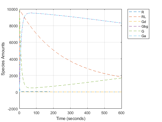
To note the fast rise and subsequent decline of the species Ga, simulate the model for 600s and store the results.

Change the StopTime of the default configuration set object from 10s (simulationTime) to 600s. In addition, don't log data for the ligand 'L' (modelObj.Species(1)) because it takes on values that are orders of magnitude higher than the other species. This makes visualizing the species in a plot more convenient. To accomplish this, define StatesToLog to include all species except 'L'.

 configsetObj = getconfigset(modelObj);
 configsetObj.StopTime = 600;
 configsetObj.SolverOptions.AbsoluteTolerance = 1.e-9;
 configsetObj.RuntimeOptions.StatesToLog = ...
     sbioselect(modelObj, 'Type', 'species', 'Where', 'Name', '~=', 'L');

Simulate the model and return the results to the three variables 'time', 'data', and 'names'.

 [time, data, names] = sbiosimulate(modelObj);

Plot the data.

 plot(time, data);
 legend(names, 'Location', 'NorthEastOutside');
 xlabel('Time (seconds)');
 ylabel('Species Amounts');
 grid on;

Creating a Model Variant for the Mutant Strain

The G-Protein cycle model for the mutant strain differs in the rate at which the inactivation of the active G-protein (Ga) takes place. This rate is governed by the value of the rate parameter kGd. You can represent the mutant strain using a Variant object. A SimBiology Variant stores alternate values for one or more properties of a SimBiology model, such as the InitialAmount of a species or the Value of a parameter.

Add a variant named 'mutant' to the model.

 variantObj = addvariant(modelObj, 'mutant');

Add content to the variant to specify an alternate value of 0.004 for the parameter kGd.

 addcontent(variantObj, {'parameter', 'kGd', 'Value', 0.004});

Simulating the Mutant Pathway and Plotting the Results

Simulate the model using the mutant variant object. This applies the value of 0.004 to the parameter kGd during simulation. Return the simulation results in a SimData object. In addition to storing SimBiology simulation data, SimData objects provide methods for data access, plotting, and analysis.

Set the Active property of the mutant variant object to true and simulate.

 variantObj.Active = true;
 mutantData = sbiosimulate(modelObj);

Plot the data using dashed lines. See also sbioplot for convenient plotting of SimData objects.

 plot(mutantData.Time, mutantData.Data, 'LineStyle', '--');
 legend(mutantData.DataNames, 'Location', 'NorthEastOutside');
 xlabel('Time (seconds)');
 ylabel('Species Amounts');
 grid on;

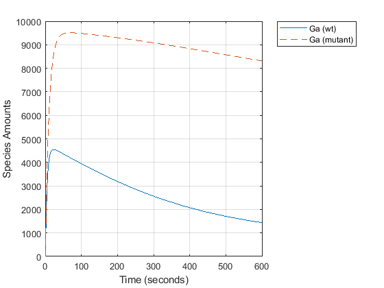
Compare the behavior of the active G-Protein species (Ga) in the wild-type and mutant pathways.

 GaIndex = strcmp(names, 'Ga'); % index for wild-type results
 [tmut, xmut] = selectbyname(mutantData, 'Ga');
 plot(time, data(:,GaIndex), tmut, xmut, '--');
 xlabel('Time (seconds)');
 ylabel('Species Amounts');
 legend({'Ga (wt)','Ga (mutant)'}, 'Location', 'NorthEastOutside');
 grid on;

Performing a Parameter Scan

The rate of G-protein inactivation is much lower in the mutant strain relative to the wild-type (kGd = 0.004 vs kGd = 0.11), which explains the higher levels of activated G-protein (Ga) over time observed in the above comparison. For a more detailed look at how the variation of kGd affects levels of Ga, perform a parameter scan of several simulations in which the value of kGd is varied over a range of values. The following example illustrates a parameter scan over five values of kGd; to increase the number of iterations, change the values in the arguments for the linspace function below.

Generate five evenly-spaced kGd values ranging from 0.001 to 0.15.

 kGdValues = linspace(1e-3, 0.15, 5);

Store the results of the parameter scan in an array of SimData objects. Initialize a variable to hold this array.

 scanData = [];

Prepare the model for accelerated simulation.

 sbioaccelerate(modelObj);

Loop over kGdValues and perform a simulation for each value. Use the mutant variant on the model to modify the value of kGd used during simulation.

for kGd = kGdValues
    % Set the desired value of kGd in the variant.
    variantObj.Content{1}{4} = kGd;

    % Simulate the model, storing the results in a SimData object.
    sd = sbiosimulate(modelObj);
    scanData = [scanData; sd];
end

scanData is now a five element array of SimData objects. Each object contains the data from one run in the parameter scan.

Extract the timecourses for Ga from the SimData object array and plot on a single axis. The following code constructs the plot step-by-step; alternatively, see sbioplot and sbiosubplot.

 [tscan, xscan] = selectbyname(scanData, 'Ga');

 fh = figure;
 hold on;
 for c = 1:5
    plot(tscan{c}, xscan{c});
    str = sprintf(' k = %5.3f', kGdValues(c));
    text(tscan{c}(end), xscan{c}(end), str);
 end

 % Annotate the plot.
 axis(gca(fh), 'square');
 title('Varying the Value of kGd: Effect on Ga');
 xlabel('Time (seconds)');
 ylabel('Species Amounts');
 grid on;
 hold off;

Parameter Estimation - Background

When modeling biological systems, it is often necessary to include parameters whose numerical value is unknown or only roughly known. If experimental data is available for one or more species in the system, the values of these parameters can be estimated by varying them and looking for those values which lead to the best fit between the model's simulated results and the experimental data.

In this section of the example we explore parameter estimation functionality in the context of trying to fit the G protein model to experimental data.

Parameter Estimation - Comparing Model Results to Experimental Data

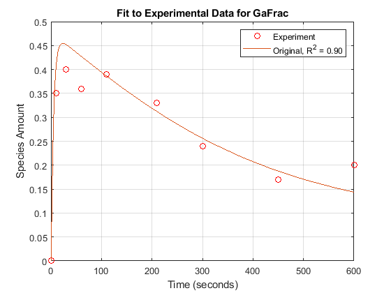
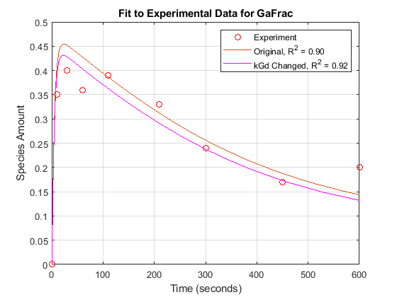
For experimental data, Fig. 5 of the reference paper contains the timecourse for the fraction of active G protein.

Store the experimental time and state data.

  tExpt = [0 10 30 60 110 210 300 450 600]';
  GaFracExpt = [0 0.35 0.4 0.36 0.39 0.33 0.24 0.17 0.2]';
  data = groupedData(table(tExpt, GaFracExpt));
  data.Properties.IndependentVariableName = 'tExpt';

Instead of converting this experimental data to absolute amounts of Ga, add this fraction to the model using a non-constant parameter and a repeatedAssignment rule.

 GaFracObj = modelObj.addparameter('GaFrac', 'ConstantValue', 0);
 GaFracRule = modelObj.addrule('GaFrac = Ga / (Ga + G + Gd)', 'repeatedAssignment')

GaFracRule = 

   SimBiology Rule Array

   Index:    RuleType:             Rule:                      
   1         repeatedAssignment    GaFrac = Ga / (Ga + G + Gd)

Change the RuntimeOptions on the configuration set to log GaFrac.

 configsetObj.RuntimeOptions.StatesToLog = GaFracObj;

Deactivate the mutant variant.

 variantObj.Active = false;

Simulate the model, storing the results in a SimData object.

 sdWild = sbiosimulate(modelObj);

Get the data for 'GaFrac' to be used later in a plot.

 [tWild, GaFracWild] = selectbyname(sdWild, 'GaFrac');

Resample the simulation results onto the experimental time vector.

 sdWildResampled = resample(sdWild, tExpt, 'pchip');

Get the resampled data for the species 'Ga'.

 [~, GaFracWildResampled] = selectbyname(sdWildResampled, 'GaFrac');

Compute the R-square value measuring the fit between the simulated and experimental data.

 sst = norm(GaFracExpt - mean(GaFracExpt))^2;
 sse = norm(GaFracExpt - GaFracWildResampled)^2;
 rSquare = 1-sse/sst;

Plot the simulation results against the experimental data for Ga.

 fh = figure;
 plot(tExpt, GaFracExpt, 'ro');
 legendText = {'Experiment'};
 title('Fit to Experimental Data for GaFrac');
 xlabel('Time (seconds)');
 ylabel('Species Amount');
 hold on;
 plot(tWild, GaFracWild);
 legendText{end+1} = sprintf('Original, R^2 = %4.2f', rSquare);
 legend(legendText{:});
 grid on;

Parameter Estimation - Estimating a Single Model Parameter

From the parameter scan, we've seen that the value of the parameter kGd has a significant effect on the timecourse of the species Ga. Let's see if we can improve the fit of the model results to the experimental data by varying the value of kGd.

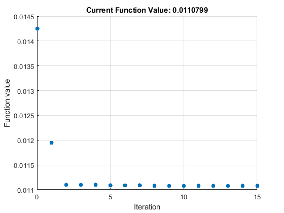
Perform parameter estimation against the experimental data, optimizing the value of kGd. Plot information about iterations while the optimization progresses, up to a maximum of 15 iterations.

 paramToEst = estimatedInfo('kGd');
 kGdObj = sbioselect(modelObj, 'Name', 'kGd');
 opt = optimset('PlotFcns',@optimplotfval,'MaxIter',15);
 result1 = sbiofit(modelObj, data, 'GaFrac = GaFracExpt', paramToEst, ...
     [], 'fminsearch', opt);
 estValues1 = result1.ParameterEstimates

estValues1 =

  1x3 table

     Name      Estimate    StandardError
    _______    ________    _____________

    {'kGd'}    0.12142       0.0018606  

Store the estimated value of kGd in a new model Variant.

 optimVariantObj = addvariant(modelObj, 'Optimized kGd');
 addcontent(optimVariantObj, {'parameter', 'kGd', 'Value', estValues1.Estimate});

Activate the new variant and inactivate the 'mutant' variant.

 optimVariantObj.Active = true;
 mutantVariantObj = getvariant(modelObj, 'mutant');
 mutantVariantObj.Active = false;

Simulate the model using the estimated value of kGd.

 sdEst1 = sbiosimulate(modelObj);

Plot the data for GaFrac and compare with the previous results.

 [t1, GaFracEst1] = selectbyname(sdEst1, 'GaFrac');
 sdEst1Resampled = resample(sdEst1, tExpt, 'pchip');
 [~, GaFracEst1Resampled] = selectbyname(sdEst1Resampled, 'GaFrac');
 sse1 = norm(GaFracExpt - GaFracEst1Resampled)^2;
 rSquare1 = 1-sse1/sst;
 figure(fh);
 plot(t1, GaFracEst1, 'm-');
 legendText{end+1} = sprintf('kGd Changed, R^2 = %4.2f', rSquare1);
 legend(legendText{:});

From the R-square values, we see that the fit to the experimental data is slightly better with the new, estimated value of kGd. If the original value for kGd was only a rough estimate, we could interpret these results either as a confirmation of the original estimate or an improvement over it.

Sensitivity Analysis - Background

So far we have been interested in the dynamic behavior of the active G protein, species Ga. A parameter scan revealed that this species is significantly affected by the value of the rate constant kGd governing G-protein inactivation. Using parameter estimation, we found that by optimizing the value of kGd, we were able to better fit an experimental timecourse for Ga.

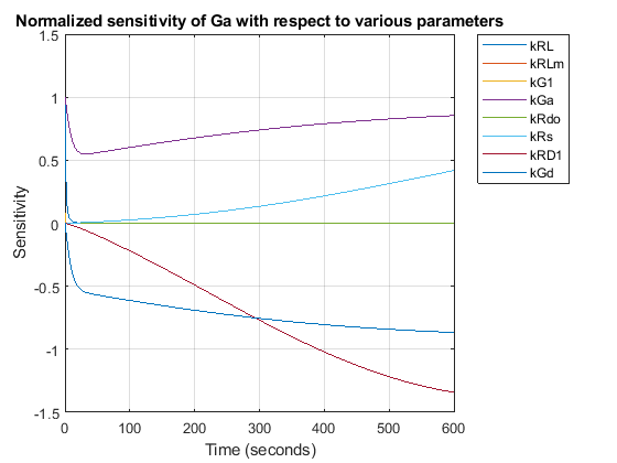
A natural question to ask is, what other parameters of the model affect Ga levels, and what are the magnitudes of those effects? Sensitivity analysis allows you to answer these questions by computing the time-dependent derivatives of one or more species ("outputs") relative to either model parameter values, or species initial conditions ("input factors").

Sensitivity Analysis - Computing Sensitivities

Compute the sensitivity of Ga with respect to various parameters in the model. Normalize the sensitivities fully so they can be compared with each other.

Deactivate the mutant variant object on the model so that sensitivities are computed with kGd at its original value.

 optimVariantObj.Active = false;

Set up the sensitivity calculation in the model configset.

% Turn on SensitivityAnalysis in the solver options.
 configsetObj.SolverOptions.SensitivityAnalysis = true;

% Configure the sensitivity outputs and inputs for sensitivity analysis.
 sensitivityOpt = configsetObj.SensitivityAnalysisOptions;
 GaObj = sbioselect(modelObj, 'Type', 'species', 'Name', 'Ga');
 sensitivityOpt.Outputs = GaObj;
 params = sbioselect(modelObj, 'Type', 'parameter', 'Where', 'Name', '~=', 'GaFrac');
 sensitivityOpt.Inputs = params;
 sensitivityOpt.Normalization = 'Full';

Simulate the model.

 sdSens = sbiosimulate(modelObj);

Extract the sensitivity data from the SimData object and plot the computed sensitivities.

 [t, R, sensOutputs, sensInputs] = getsensmatrix(sdSens);
 R = squeeze(R);

 figure;
 plot(t,R);
 title('Normalized sensitivity of Ga with respect to various parameters');
 xlabel('Time (seconds)');
 ylabel('Sensitivity');
 legend(sensInputs, 'Location', 'NorthEastOutside');
 grid on;

Parameter Estimation - Estimating Multiple Parameters

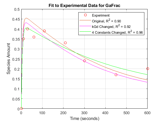
These results show that Ga is not only sensitive to the parameter kGd, but also to kGa, kRs, and kRD1. (The other sensitivities are indistinguishable from zero on the plot.) Varying these four parameters may make the fit to experimental data better still.

Estimate these four parameters to match the target data. Use the previously configured optimization options and the current parameter values in the model as the starting point for optimization.

Select the parameters kGa, kRs, kRD1, and kGd for estimation.

 paramsToEst = estimatedInfo({'kGa', 'kRs', 'kRD1', 'kGd'});

Parameter estimation will ignore the sensitivity analysis option if it is enabled in the configset. Turn off SensitivityAnalysis in the solver options to avoid warnings.

 configsetObj.SolverOptions.SensitivityAnalysis = false;
 result2 = sbiofit(modelObj, data, 'GaFrac = GaFracExpt', paramsToEst, ...
     [], 'fminsearch', opt);
 estValues2 = result2.ParameterEstimates

estValues2 =

  4x3 table

      Name       Estimate     StandardError
    ________    __________    _____________

    {'kGa' }    9.0068e-06     3.0255e-06  
    {'kRs' }         4.549          11.76  
    {'kRD1'}     0.0031018       0.002734  
    {'kGd' }       0.12381       0.053693  

Store the estimated values of the four parameters in a new model variant.

 optimVariantObj2 = addvariant(modelObj, 'Four parameter optimization');
 addcontent(optimVariantObj2, {'parameter','kGa', 'Value', estValues2.Estimate(1)});
 addcontent(optimVariantObj2, {'parameter','kRs', 'Value', estValues2.Estimate(2)});
 addcontent(optimVariantObj2, {'parameter','kRD1','Value', estValues2.Estimate(3)});
 addcontent(optimVariantObj2, {'parameter','kGd', 'Value', estValues2.Estimate(4)});

Now simulate the model with the newly estimated parameter values.

 optimVariantObj.Active = false;
 optimVariantObj2.Active = true;
 sdEst2 = sbiosimulate(modelObj);

Compare with the previous results.

 [t2, GaFracEst2] = selectbyname(sdEst2, 'GaFrac');
 sdEst2Resampled = resample(sdEst2, tExpt, 'pchip');
 [~, GaFracEst2Resampled] = selectbyname(sdEst2Resampled, 'GaFrac');
 sse2 = norm(GaFracExpt - GaFracEst2Resampled)^2;
 rSquare2 = 1-sse2/sst;
 figure(fh);
 plot(t2, GaFracEst2, 'g-');
 legendText{end+1} = sprintf('4 Constants Changed, R^2 = %4.2f', rSquare2);
 legend(legendText{:});

With parameter estimation free to vary four parameters, the fit to experimental data has improved further. The displayed optimization iterations show that the objective function has decreased and the R-square value has increased.

Note that the four-parameter estimation performed here may or may not be biologically relevant and is for illustrative purposes only.

Note also that storing the estimation results in variants makes it easy to switch back and forth between simulating different versions of the model. There are four versions at this point: the original, the mutant, and two versions based on the results of parameter estimations.

Conclusion

This example introduced various aspects of SimBiology functionality for model building, simulation, and analysis using a model of G protein signaling.