Stochastic Simulation of Radioactive Decay
This example shows how to build and simulate a model using the SSA stochastic solver.
The following model will be constructed and stochastically simulated:
Reaction 1: x -> z with a first-order reaction rate, c = 0.5.
Initial conditions: x = 1000 molecules, z = 0.
This model can also be used to represent irreversible isomerization.
This example uses parameters and conditions as described in Daniel T. Gillespie, 1977, "Exact Stochastic Simulation of Coupled Chemical Reactions," The Journal of Physical Chemistry, vol. 81, no. 25, pp. 2340-2361.
Read the Radioactive Decay Model Saved in SBML Format
model = sbmlimport('radiodecay.xml')model =
SimBiology Model - RadioactiveDecay
Model Components:
Compartments: 1
Events: 0
Parameters: 1
Reactions: 1
Rules: 0
Species: 2
Observables: 0
View Species Objects of the Model
model.Species
ans =
   SimBiology Species Array

   Index:    Compartment:    Name:    Value:    Units:
   1         unnamed         x        1000      molecule
   2         unnamed         z        0         molecule
View Reaction Objects of the Model
model.Reactions
ans =
   SimBiology Reaction Array

   Index:    Reaction:
   1         x -> z
View Parameter Objects for the Kinetic Law
model.Reactions(1).KineticLaw(1).Parameters
ans =
   SimBiology Parameter Array

   Index:    Name:    Value:    Units:
   1         c        0.5       1/second
Update the Reaction to use MassAction Kinetic Law for Stochastic Solvers.
model.Reactions(1).KineticLaw(1).KineticLawName = 'MassAction';
model.Reactions(1).KineticLaw(1).ParameterVariableNames = {'c'};
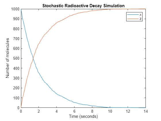
Simulate the Model Using the Stochastic (SSA) Solver & Plot
cs = getconfigset(model,'active');
cs.SolverType = 'ssa';
cs.StopTime = 14.0;
cs.CompileOptions.DimensionalAnalysis = false;
[t,X] = sbiosimulate(model);

plot(t,X);
legend('x', 'z', 'AutoUpdate', 'off');
title('Stochastic Radioactive Decay Simulation');
ylabel('Number of molecules');
xlabel('Time (seconds)');
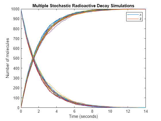
Repeat the Simulation to Show Run-to-Run Variability
title('Multiple Stochastic Radioactive Decay Simulations');
hold on;
for loop = 1:20
    [t,X] = sbiosimulate(model);
    plot(t,X);    % Just plot number of reactant molecules
    drawnow;
end
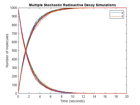
Overlay the Reaction's ODE Solution in Red
cs = getconfigset(model,'active');
cs.SolverType = 'sundials';
cs.StopTime = 20;
[t,X] = sbiosimulate(model);
plot(t,X,'red');
hold off;