Job Scheduling and Resource Estimation for a Manufacturing Plant

Overview

This example shows you how to model a manufacturing plant. The plant consists of an assembly line that processes jobs based on a pre-determined schedule. This example walks you through a workflow for:

Structure of the Model

The manufacturing plant caters to the production of 40 different product variants based on pre-defined schedules. Each variant requires two parts, PartA and PartB that correspond to that particular variant. Each part goes through a sequence of manufacturing steps. The following modeling details are specified in an Excel file that are read during model initialization:

The following script reads the excel file and initializes all the parameters.

modelname = 'seEstimatingAssemblyLineThroughput';
open_system(modelname);
scopes = find_system(modelname,'LookUnderMasks','on','BlockType','Scope');
cellfun(@(x)close_system(x), scopes);

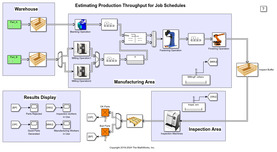
The manufacturing plant mainly consists of two areas:

The Manufacturing area: The plant receives job orders that are to be fulfilled. A job order specifies the variant ID and the required quantity for that particular variant. The Entity Generators generate parts based on a pre-defined sequence that satisfies the job order. In this example the sequence is either generated from a MATLAB script or is read from the excel sheet. The following script reads the job order requirements from the excel file.

To manufacture a particular variant, PartA and PartB that correspond to the variant are brought in together into the manufacturing area. The parts go through the following steps before leaving the manufacturing area:

Average operation completion times for each variant are tabulated in the excel sheet. A 4% variation in operation completion times is assumed. Workers from the manufacturing worker pool load and unload parts from the Milling and Fastening machines.

open_system([modelname '/Milling Operation1']);

close_system([modelname '/Milling Operation1']);

The Inspection area: The finished product enters the Inspection area, where the product is either certified to be ok or is rejected and scrapped. This example assumes a 5% rejection rate in the inspection area. Workers from the inspection worker pool load and unload parts from the three inspection machines.

open_system([modelname '/Inspection Machines']);

close_system([modelname '/Inspection Machines']);

Analyzing The Impact of Job Schedule on Throughput

To meet the job order requirements with the best throughput, different schedules can be generated. In this example, throughput is the total number of good products produced by the plant. The sheet named 'MfgSchedule' shows a few schedules that satisfy the job order. Following scripts generate job schedules based on certain criteria:

This schedule puts the operation having shortest running time on the Blanking machine first and the longest one at the end. The idea here is to push as many parts into the plant as early as possible. The throughput is then examined:

idx = 1;
S1 = sortrows(optimes(:, [1 2]), 2);
for i = 1:length(S1)
    repeat = requirements(S1(i), 2);
    for j = 1:repeat
        newSchedule(idx) = S1(i);
        idx = idx + 1;
    end
end
scheduleID = size(schedule, 2) + 1;
schedule(:, scheduleID) = newSchedule';
sim(modelname);
open_system([modelname '/Good Parts Generated']);

close_system([modelname '/Good Parts Generated']);

This schedule puts the operation having the shortest running time on the Milling machines first and the longest one at the end. The idea again is to push as many parts into the plant as early as possible from the other starting branch of the plant. The throughput is then examined:

idx = 1;
S2 = sortrows(optimes(:, [1 3]), 2);
for i = 1:length(S2)
    repeat = requirements(S2(i), 2);
    for j = 1:repeat
        newSchedule(idx) = S2(i);
        idx = idx + 1;
    end
end
scheduleID = size(schedule, 2) + 1;
schedule(:, scheduleID) = newSchedule';
sim(modelname);
open_system([modelname '/Good Parts Generated']);

close_system([modelname '/Good Parts Generated']);

This schedule puts the operation having shortest running time on the Fastening machine first and the longest one at the end. The idea here is to push parts out of the bottleneck machine as early as possible. The throughput is then examined:

idx = 1;
S4 = sortrows(optimes(:, [1 5]), 2);
for i = 1:length(S4)
    repeat = requirements(S4(i), 2);
    for j = 1:repeat
        newSchedule(idx) = S4(i);
        idx = idx + 1;
    end
end
scheduleID = size(schedule, 2) + 1;
schedule(:, scheduleID) = newSchedule';
sim(modelname);
open_system([modelname '/Good Parts Generated']);

close_system([modelname '/Good Parts Generated']);%%

This schedule takes into account the cumulative run time on all the machines. The operation having the shortest cumulative run time is put first and the longest one goes to the end. The throughput is then examined:

idx = 1;
cumulativeSum = sortrows([optimes(:, 1) sum(optimes(:, [2 3 5 6]), 2)], 2);
for i=1:length(cumulativeSum)
    repeat = requirements(cumulativeSum(i), 2);
    for j = 1:repeat
        newSchedule(idx) = cumulativeSum(i);
        idx = idx + 1;
    end
end
scheduleID = size(schedule, 2) + 1;
schedule(:, scheduleID) = newSchedule';

sim(modelname);
open_system([modelname '/Good Parts Generated']);

close_system([modelname '/Good Parts Generated']);

Schedules 5 to 8 in the excel sheet are all random schedules which satisfy the job order. These schedules can be generated by starting from any schedule and generating a random permutation using the RANDPERM function. Following are the results for 'Schedule 8':

scheduleID = 9;
sim(modelname);
open_system([modelname '/Good Parts Generated']);

close_system([modelname '/Good Parts Generated']);

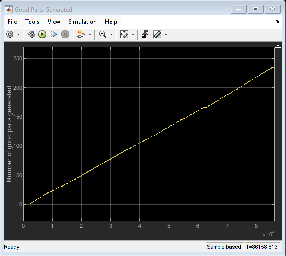
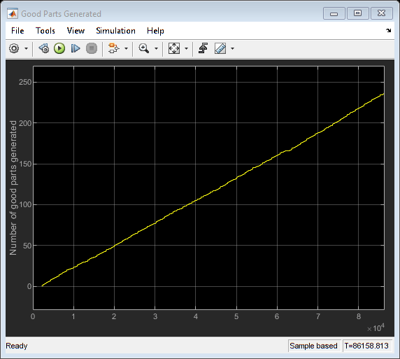
Simulating all of the above strategies suggests that the schedule associated with 'Shortest job first on the Fastening Machine', 'Schedule 3' gives us the best throughput.

Estimating the Number of Workers

After selecting the best schedule, an estimate of the number of workers needed in the two worker pools is made. We start with three workers working in the Manufacturing area and three in the Inspection area.

numMfgWorkers = 3;
numInspectWorkers = 3;
sim(modelname);
open_system([modelname '/Manufacturing Workers in Use']);
open_system([modelname '/Inspection workers in Use']);
open_system([modelname '/Good Parts Generated']);

close_system([modelname '/Manufacturing Workers in Use']);
close_system([modelname '/Inspection workers in Use']);
close_system([modelname '/Good Parts Generated']);

From the scopes we see that the maximum number of workers in the Manufacturing and Inspection pools used at any given point in time rarely exceeds two. Reducing the number of workers to two shows that there is no impact on throughput with better worker utilization.

numMfgWorkers = 2;
numInspectWorkers = 2;

sim(modelname);
open_system([modelname '/Manufacturing Workers in Use']);
open_system([modelname '/Inspection workers in Use']);
open_system([modelname '/Good Parts Generated']);

close_system([modelname '/Manufacturing Workers in Use']);
close_system([modelname '/Inspection workers in Use']);

close_system([modelname '/Good Parts Generated']);

Conclusion

This example shows how we can use SimEvents to model a job shop. The use of MATLAB scripts allows us to experiment and arrive at the best schedule.

% The following script closes and cleans up the model
bdclose(modelname);
clear numMfgWorkers numInspectWorkers modelname  ...
    scheduleID discard_rate scopes schedule requirements ...
	 optimes ;