Model Simple Order Fulfilment Using Autonomous Robots
This example models a warehouse with autonomous robots for order management. The goal of the example is to show how to facilitate complex models created with Simulink®, Stateflow®, and SimEvents® components and their communication via messages. See View Differences Between Stateflow Messages, Events, and Data (Stateflow) for more information about messages.
Order Fulfilment Model
Order fulfilment model has two major components
The Order Queue component represents an online order queue with the blocks from the SimEvents® library.
The Warehouse component represents delivery of order items by autonomous robots. It uses blocks from Simulink® and SimEvents® libraries and a Stateflow® chart. The chart requires a Stateflow® license.
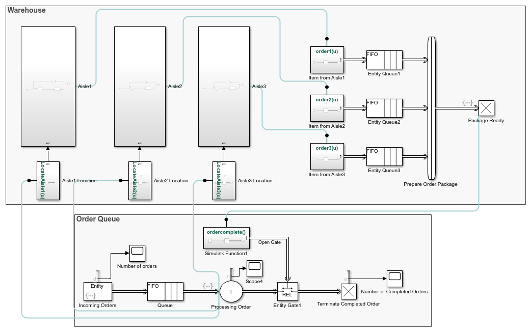
In this model, an online order for multiple items arrives at the Order Queue component. The locations of the ordered items are communicated from the Processing Order block to the autonomous robots in the Warehouse component. Three robots are assigned to three aisles. A robot picks up an item from its aisle location and returns it to its initial location for delivery. An order can have one, two, or three items. When all ordered items are delivered by the robots, the order is complete and a new order arrives. Until an order is complete, no new orders are received to the Order Queue component.
Warehouse Component
The warehouse has three aisles. The first aisle contains clothing items, the second aisle contains toys, and the third aisle contains electronics. Three delivery robots are identical and their dynamics are driven by a linear time-invariant system that is controlled by a tuned PID controller. For instance, the Aisle1 subsystem block consists of a Robot1 subsystem and a Discrete-Event Chart block as a scheduler.

Robot1 Subsystem
The Robot1 subsystem has a generic feedback control loop with the dynamics of the robot represented by the State-Space block and the PID controller.

The Robot1 subsystem is designed to track a reference signal from the
In1 block, which is the out signal from
the Discrete-Event Chart block. The system compares the input
value with the output from the State-Space block and the
difference between signals is fed to the PID Controller
block.
For instance, if the signal from the In1 block is a constant
with value 10, starting from the initial state
0, the output of the system converges to
10.
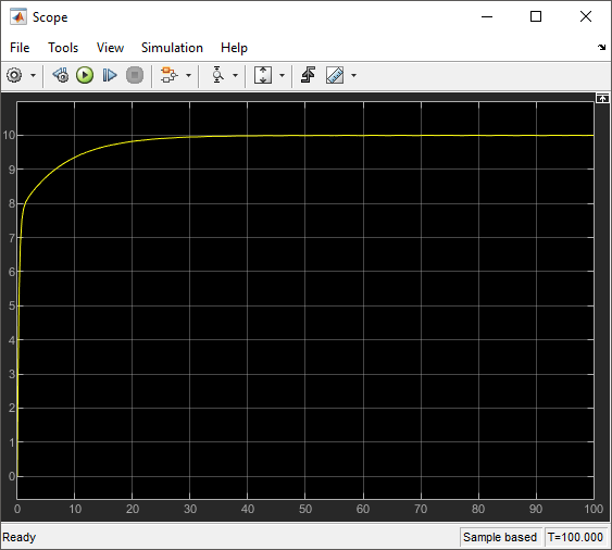
In the x-axis and y-axis, Robot1 moves as follows.
Robot1 is initially at x1 and y1 = 0 coordinate. For item pickup and delivery, it moves only on the y-axis and its x1 coordinate remains the same.
Each order item in Aisle1 has a yaisle coordinate on the y-axis. yaisle becomes the constant input reference signal to be tracked by Robot1 subsystem.
When Robot1 subsystem reaches yaisle, it picks up the order item and autonomously reruns back to y1 = 0 location for delivery.
The scope displays an example trajectory for Robot1 subsystem, which receives
a yaisle value 10 as the constant
reference input at simulation time 265. When the distance
between the robot's location and y = 10 is 0.1, reference input signal is
0 and the robot returns to its initial location for
delivery.
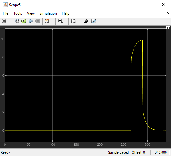
Robot2 subsystem and Robot3 subsystem have identical dynamics and behavior for the item delivery in Aisle2 subsystem and Aisle3 subsystem. Their x coordinates are x2 and x3 and they also move on the vertical y-axis.
Scheduler
In the previous example trajectory, Robot1 has three states. The Discrete-Event Chart block is used to schedule the transitions between these robot states.
A robot waits in the
Waitstate, until it receives a yaisle item coordinate. Robot1 subsystem is in theWaitstate, until the simulation time is265.A robot transitions to the
PickUpstate, when there is an incoming message carrying the yaisle value of an item to the Discrete-Event Chart block. This value is assigned toout, which is the output signal from the Discrete-Event Chart block. Theoutsignal is fed to the Robot1 subsystem as the input signal In1 to be tracked and the robot moves towards the yaisle item location. Robot1 subsystem transitions to thePickUpstate at time265.When a robot is
0.1units away from yaisle, it picks up the item. Then, the robot transitions to aDeliverstate. Theoutsignal becomes0and the robot returns back to y = 0 for delivery. At the simulation time290, Robot1 subsystem is0.1unit away from y = 10 and transitions to theDeliverstate.When a robot returns and it is
0.1units away from y = 0, it transitions to theWaitstate. At around320, Robot1 subsystem delivers the item and transitions back to theWaitstate.
![Snapshot of the Discrete-Event Chart block showing transitions between the three states of the robot: Wait, PickUp and Deliver. The transition condition from the Wait state to the PickUp state is: yaisle{target = yaisle.data;out=target;}. The transition condition from the PickUp state to the Deliver state is: [abs(y-target)<0.1]{out=0;}. The transition condition from the Deliver state to the Wait state is: [y<0.1]{order1(1);}.](warehouse_chart.png)
Order Package Preparation
When a robot delivers its item, the item is sent to generate the order package. This behavior is represented by the Message Send block that generates a message inside the Item from Aisle Simulink Function block. Then, the generated message enters the Entity Queue block.
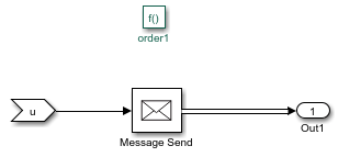
A Composite Entity Creator block waits for all three items from the three Entity Queue blocks to create a composite entity that represents the order.
To complete the order, all of the items from the three aisles are required to be delivered.
When all the items are delivered, the order is complete and it arrives at the Package Ready block.
The entry of the order to the Package Ready block triggers the Simulink Function1 block to generate a message and to open the gate for order termination.
When the order is terminated, a new order arrives at the Processing Order block which restarts the delivery process.
Until an order is complete, no new orders are received, so the robots that deliver their items wait for the order to be completed.
Order Queue Component
The order queue block is a simple queuing system composed of an Entity Generator, Entity Queue, Entity Server, Entity Gate, and Entity Terminator block. For more information about creating a simple queuing system, see Manage Entities Using Event Actions.
Entity Generator block randomly generates orders. The intergeneration time is drawn from an exponential distribution with mean
100.Each generated entity has three randomly generated attributes
aisle1,aisle2, andaisle3that represent the yaisle coordinates of the items in Aisle1, Aisle2, and Aisle3 subsystems.entity.Aisle1 = randi([1,30]); entity.Aisle2 = randi([1,30]); entity.Aisle3 = randi([1,30]);
It is assumed that the items are located vertically between y = 1 and y = 30.
The arrival of the order to the Entity Server block activates the robots by communicating the items' yaisle coordinates. Entering this MATLAB® code in the Entry action field.
LocateAisle1(entity.Aisle1);
LocateAisle2(entity.Aisle2);
LocateAisle3(entity.Aisle3);
Calling the
LocateIsle()function communicates the yaisle coordinate of an item to the corresponding robot.The order waits in the Entity Server block until the Entity Gate block opens.
When all items are delivered, the order package enters the Package Ready block and its entry calls the Simulink Function1 block through the function
ordercomplete(). The Simulink Function1 block generates a message to open the gate.When the gate opens, the order is terminated and a new order arrives at the Entity Server block.
Results
Inspect the order throughput from the Order Queue.
Increase the simulation time to
1000.Simulate the model and observe that the scope displays
7as the total number of completed orders.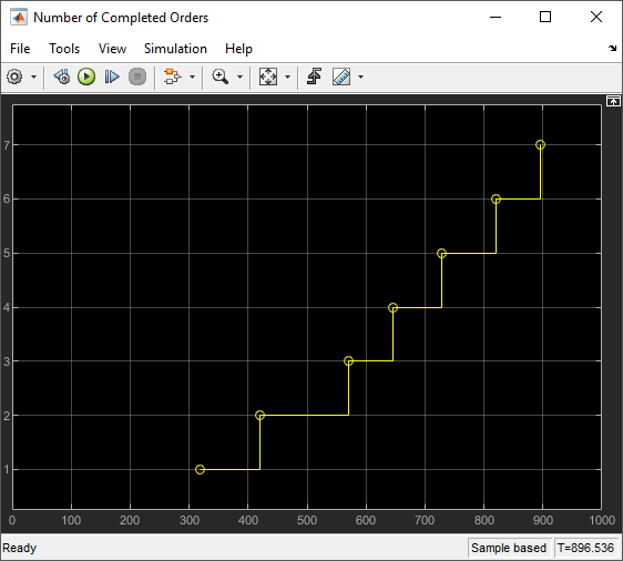
See Also
Entity Server | Entity Generator | Queue | Entity Terminator | Discrete-Event Chart