Optimization of Shared Resources in a Batch Production Process

Overview

This example shows how to model and optimize the use of shared resources in a system, to identify resource deficiencies and improve capacity planning. The example is based on a batch production process, where production orders are processed only according to the availability of batch reactors. In the example, SimEvents® entities represent both the production orders of the manufacturing process, and the batch reactors that are required to process them. Later in the example, we will find the optimal resource capacities of the system by applying the Genetic Algorithm solver of MATLAB Global Optimization Toolbox.

modelname = 'seBatchProduction';
open_system(modelname);
scopes = find_system(modelname, 'LookUnderMasks', 'on', 'BlockType', 'Scope');
cellfun(@(x)close_system(x), scopes);
set_param(modelname, 'SimulationCommand', 'update');

Structure of Model

At the top level of the model, the Entity Generators simulate the generation and backlog of production orders by generating entities that represent production orders. When a new entity is generated, the Obtain Reactor block requests a batch reactor to process the order. After the Execute Chemical Process Recipe subsystem completes the order according to a specified chemical process recipe, the block labeled Release Reactor releases the batch reactor back into the pool of resources, where it is now available to process a new order. The Data Analysis subsystem analyzes data related to completion of production orders.

Shared Resources in the Production Process

The Execute Chemical Process Recipe subsystem simulates the chemical process to produce sol (a type of colloid). A six-step recipe models the main operations in sol production. Execution of these steps requires different resources. A batch reactor provides built-in capabilities to execute steps like adding color, adding particles and stir. Thus the resources required by these steps do not need to be modeled separately. On the other hand, the steps to add water, heat up and drain require extra resources. These resources are shared by all the batch reactors and are limited by the capacity of the production system.

open_system([modelname '/Execute Chemical Process Recipe']);

For example, when water usage reaches the full capacity, water pressure is too low for another batch reactor to access. In this case, production in that reactor pauses until the water supply becomes available again. In the Execute Chemical Process Recipe subsystem, the example models such a resource sharing process with a Queue block labeled Wait for Water Supply and an Entity Server block labeled Add Water in the Add Water subsystem. The Capacity parameter of the Entity Server block models the capacity of the water supply. During simulation, the number of entities in the Queue block indicates the number of batch reactors waiting for water. The number of entities in the Server block represents the number of batch reactors accessing water.

open_system([modelname '/Execute Chemical Process Recipe/Add Water']);

The modeled batch production process is capable of producing two types of batches: type A and type B. Although the main steps required to produce either batch are the same, the chemical process recipes are different. For example, the recipe to produce type B requires more water, so the step to add water takes more time to complete.

Results and Displays

During simulation, the Data Analysis subsystem displays several results to show the performance of the production process.

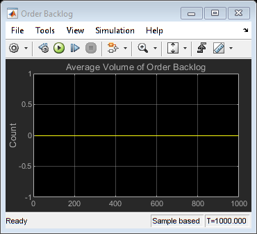
The most illustrative result here is the first one, Average number of orders in backlog, which represents the wait time for orders as the system struggles to keep up with inflow.

sim(modelname);
open_system([modelname '/Data Analysis/Order Backlog']);

Other results of the system include the following and can be seen in the Data Analysis subsystem:

open_system([modelname '/Data Analysis/Waiting For Water']);
open_system([modelname '/Data Analysis/Waiting For Heat']);
open_system([modelname '/Data Analysis/Waiting For Drain']);
open_system([modelname '/Data Analysis/Utilization Reactors']);
open_system([modelname '/Data Analysis/Utilization Water']);
open_system([modelname '/Data Analysis/Utilization Heaters']);
open_system([modelname '/Data Analysis/Utilization Drains']);
open_system([modelname '/Data Analysis/ThroughputA']);
open_system([modelname '/Data Analysis/ThroughputB']);

Optimizing Resource Capacities

We will now apply a Genetic Algorithm solver from the MATLAB Global Optimization Toolbox to this SimEvents model to find optimal resource capacities for this system. The genetic algorithm solves optimization problems by repeatedly modifying a population of individual points. Due to its random nature, the genetic algorithm improves your chances of finding a global solution. It does not require the functions to be differentiable or continuous.

The decision variables in this optimization are:

The genetic algorithm sets these variables as it runs multiple simulations of the model via the variable ResourceCapacity. The starting values of resource capacities are shown below:

cellfun(@(x)close_system(x), scopes);

disp('ResourceCapacity before optimization =');
disp(ResourceCapacity);
close_system([modelname '/Data Analysis/Order Backlog']);
ResourceCapacity = seRunOptimizationForBatchProductionProcess();
disp('ResourceCapacity after optimization =');
disp(ResourceCapacity);

ResourceCapacity before optimization =
     2     2     2     2

Starting parallel pool (parpool) using the 'local' profile ...
Connected to the parallel pool (number of workers: 6).
Optimization terminated: average change in the penalty fitness value less than options.FunctionTolerance
and constraint violation is less than options.ConstraintTolerance.
Elapsed time is 112.822855 seconds.
Parallel pool using the 'local' profile is shutting down.
ResourceCapacity after optimization =
    13     2     4     2

Apply Optimization Results

We can now resimulate after applying the results of the optimization process back to the model to see that this significantly reduced the order backlog.

sim(modelname);
open_system([modelname '/Data Analysis/Order Backlog']);

%cleanup
bdclose(modelname);
clear model scopes