Model RF Systems with Antenna Arrays Using RF Blockset Antenna Block
This example shows how to model MIMO receiving and transmitting RF systems including antenna arrays. The design starts from the budget analysis of a single RF chain, and it is then extended to multiple antennas. The RF Blockset™ Antenna block performs full-wave analysis of the antenna array, enabling high-fidelity modeling of the effects and imperfections coupled with the simulation of the RF system.
In the following sections, you design a MIMO receiver starting from its RF budget analysis. Then, you design a transmitter and connect the two. As a final step, the models are used to transmit and receive a wideband 100 MHZ OFDM signal, including beamsteering and clock recovery.
MIMO Receiver System
Design a MIMO receiver (RX) system starting with the budget analysis of a single antenna RF chain. In this example, the input signal is centered around 35GHz, and it is generated by a transmitter (TX) with effective isotropic radiated power (EIRP) equal to 20 dBm, located at a distance of 100 wavelengths away from the receiver.
TX_EIRP = 20;
CF = 35e9;
lambda = physconst('lightspeed')/CF; % Wavelength (m)
d = 100*lambda; % Distance between TX and RX antennas (m)
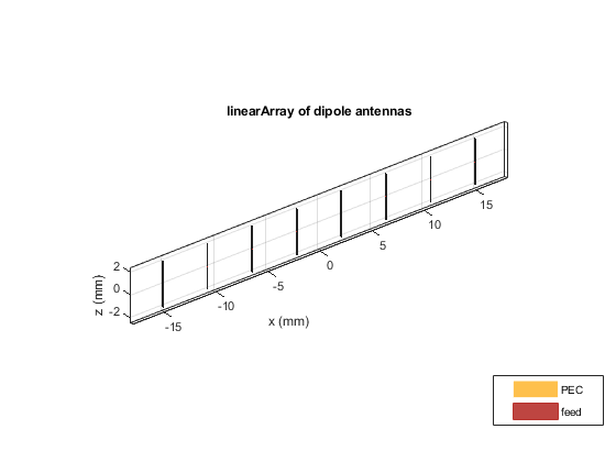
The RX array is made of eight dipole antennas located at a distance of half a wavelength from each other.
arrayRXObj = design(linearArray, CF, dipole);
arrayRXObj.NumElements = 8;
arrayRXObj.show;
Assume that the TX antenna is similar to the RX antenna and located on the same elevation plane and such that the direction of arrival is normal to the RX array axis.
DOA = 0;
Az_RX = 90-DOA; % Azimuth of direction of arrival
El_RX = 0; % Elevation of direction of arrival
First calculate the array gain using full-wave analysis, and then approximate the single antenna gain to be equal to entire array gain divided by number of elements in the array, in this case 8.
GAntRX = pattern(arrayRXObj,CF,Az_RX,El_RX, 'Type','gain');
GSingleAntRX = GAntRX - 10*log10(8);
The next element in the receiver chain is a low noise amplifier. Calculate the input impedance of the amplifier using its S-parameters interpolated at the center frequency. Note that the Touchstone file also includes the noise data.
s_amp = sparameters('amplifier.s2p');
Zin = gamma2z(gammain(rfinterp1(s_amp,CF),50));
Next, compute the impedance of the first antenna element of the array using the impedance of the amplifier determined at the previous step as load to the remaining antenna elements.
sp = sparameters(arrayRXObj,CF);
gammaInAnt1 = snp2smp(sp.Parameters,50,1,Zin);
ZAnt_RX = gamma2z(gammaInAnt1);
Calculate the free space path loss between the TX and RX.
PL = 20*log10(4*pi*d/lambda);
If the TX and RX are not perfectly aligned on the same array normal (DOA  0), the 8 received signals have different phases. To coherently receive the transmitted signal, phase shifts are needed for aligning the array beam with the direction of arrival of the received signal. The phase shift beamformer object from Phased Array System Toolbox™ is used to compute the necessary phase shifts.
Beam_Az_RX = DOA; % Beamforming angle (deg)
beamformer = phased.PhaseShiftBeamformer(...
   'SensorArray',phased.ULA('NumElements',8,...
   'ElementSpacing', lambda/2), ...
   'OperatingFrequency',CF,...
   'Direction',[Beam_Az_RX; 0],...
   'WeightsOutputPort',true);
[~, phase_shifts_RX] = beamformer(ones(1,8));
phase_shifts_RX = angle(phase_shifts_RX)'/pi*180;
Define the third-order output intercept point in dBm of the first amplifier stage in the RX chain.
oIP3_RX = 25.5;
Include an additional amplifier stage to each chain in the RX system.
G_RX = zeros(1,8);
Build a cascade (row vector) of RF receiver elements:
Antenna defined by gain and impedance, also including TX EIRP and path loss
Low noise amplifier defined by S-parameters (including noise data) and OIP3
IF Demodulator stage defined by gain and noise figure
Additional amplifier stage
Phase shifters for beamforming
% Antenna
elementsRX(1) = rfantenna( ...
    'Type','Receiver', ...
    'Gain',GSingleAntRX, ...
    'Z',ZAnt_RX, ...
    'PathLoss',PL, ...
    'TxEIRP',TX_EIRP);
% Front-end amplifier
elementsRX(2) = amplifier( ...
    'FileName','amplifier.s2p', ...
    'OIP3',oIP3_RX);
% Demodulator
elementsRX(3) = modulator( ...
    'Name','Demodulator', ...
    'Gain',-3, ...
    'NF',8, ...
    'LO',CF-100e6, ...
    'ConverterType','Down');
% Additional amplifier
elementsRX(4) = amplifier( ...
    'Gain',G_RX(1));
% Phase shifter:
elementsRX(5) = phaseshift( ...
    'PhaseShift',phase_shifts_RX(1));
Construct an rfbudget object from the above elements at the command line.
b = rfbudget( ...
    'Elements',elementsRX, ...
    'InputFrequency',CF, ...
    'SignalBandwidth',100e6, ...
    'Solver','Friis');
Type show(b) command at the command line to visualize the chain in the RF Budget Analyzer app.
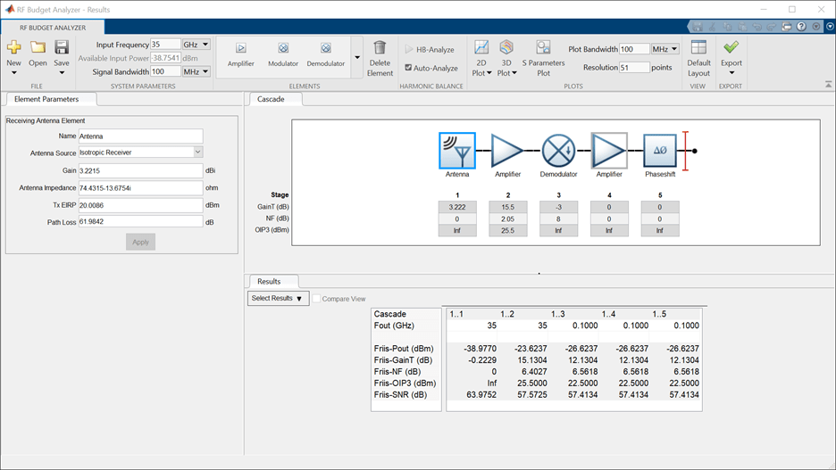
Note that the Available input power, shown in the System parameters section of the app toolstrip, is obtained by adding the transmitter EIRP, minus the path-loss plus the gain of the antenna.
Pav = TX_EIRP - PL + GSingleAntRX
Pav =

  -38.7651
Create RF Blockset Model for Receiving System
You can export the above cascade as an RF Blockset™ model and copy it to create an eight-chain RF system. When simulating the MIMO RX system, the coupling between antenna elements are captured by replacing the single antenna element used in the RF budget with a full antenna array. This is done by using an Antenna block with the antenna array object arrayRXObj.
The input to the Antenna block is the received signal described as a normalized power wave split onto the two ![$[\theta,\phi]$](../../examples/simrf/win64/ModelingRFSystemsWithAntennaArraysUsingAntennaBlockExample_eq07622708148686318631.png) polarization components. The received power wave, RX, is normalized such that the total power is
polarization components. The received power wave, RX, is normalized such that the total power is  . The antenna elements in
 arrayRXObj, are z-directed dipoles. Such an array creates a field that is polarized along the  direction. Assuming that the TX antenna array and the RX antenna array are of the same type, it can assume that the received signal is cast along the
  polarization component.
pol = [-1;0];
The resulting RX MIMO model includes an antenna block connected to a subsystem RF Receiver representing the RX system, including the eight chains:
model = 'simrfV2_RX_array';
open_system(model)
sim(model)
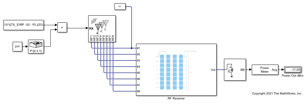
Note that the input signal is a three-dimensional array: the first dimension is used to frame data, the second dimension is used for multi-carrier signals, and the third dimension is used to provide the two polarization components.
Looking under the mask of the RF Receiver subsystem shows the structure of the multichain RF system. Each chain ends with a phase shifter, such that when the signals are combined, the array beam is aimed at the given direction of arrival. The signals are combined using inverted Wilkinson power dividers.
open_system([model '/RF Receiver'],'force');
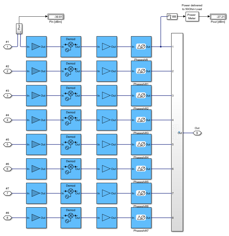
The power delivered at the input (Pin) and the output (Pout) of the first chain are measured in the model and correspond approximately to the expected values. Pout is close to the value anticipated by the analysis computed with the RF Budget Analyzer app as shown above. Pin is close to the delivered power calculated using the antenna impedance matching efficiency,  , as follows:
etaZ = 10*log10(1-abs((Zin-ZAnt_RX')/(Zin+ZAnt_RX))^2);
Pin_RX = Pav + etaZ
Pin_RX =

  -39.2525
The difference between the simulation results and the expected values computed with the budget analysis are due the approximation of the gain of the antenna element in the single RX chain as the gain of the antenna array divided by 8. This approximation ignores differences between the power received by different antenna elements in a finite array.
Close the RX model and proceed to model the TX.
bdclose(model)
MIMO Transmitter System
Design a MIMO transmitter (TX) system starting with the budget analysis of a single antenna RF chain. For MIMO transmitter system, assume an input power of -7.41 dBm and the same center frequency as the receiver.
TX_Pin = -7.41; % Transmitter input power (dBm)
DOD = 180; % Direction of departure (deg)
Design the TX antenna to be identical to the RX antenna. The array orientation is such that the direction of departure is normal to the array axis, and flipped by 180 degrees compared to the RX antenna. While this rotation does not play an important role for the current array due to symmetry along the z-axis, it might be important for other types of antennas.
arrayTXObj = design(linearArray, CF, dipole);
arrayTXObj.NumElements = 8;
arrayTXObj.TiltAxis = [0 0 1];
arrayTXObj.Tilt = 180;
The TX array is located on the same elevation plane as the RX antenna, and the direction of departure is along the array normal.
Az_TX = 90-DOD; % Azimuth direction of departure
El_TX = 0; % Elevation of direction of departure
Calculate the TX antenna array gain using full-wave analysis.
GAntTX = pattern(arrayTXObj,CF,Az_TX,El_TX, 'Type','gain');
The last stage of the TX before the antenna is a power amplifier with input and output impedance equal to 50 Ohm. Calculate the antenna impedance of the first chain of the transmitter.
Zout = 50;
sp = sparameters(arrayTXObj,CF);
gammaInAnt1 = snp2smp(sp.Parameters,50,1,Zout);
ZAnt_TX = gamma2z(gammaInAnt1);
If the TX and RX are not perfectly aligned on the same array normal (DOD 0), the 8 transmitted signals have different phases. To make sure that the transmitter steer the beam towards the receiver, phase shifts are used. Use the phase shift beamformer object from Phased Array System Toolbox to calculate the phase shifts needed for aligning the array beam with direction of arrival of the received signal.
Beam_Az_TX = DOD; % Beamforming angle (deg)
beamformer = phased.PhaseShiftBeamformer(...
   'SensorArray',phased.ULA('NumElements',8,...
   'ElementSpacing', lambda/2), ...
   'OperatingFrequency',CF,...
   'Direction',[Beam_Az_TX; 0],...
   'WeightsOutputPort',true);
[~, phase_shifts_TX] = beamformer(ones(1,8));
phase_shifts_TX = angle(phase_shifts_TX)'/pi*180;
Define the gain and third order non-linearity of the power amplifier. Add a fixed gain to each element in the TX antenna array, and define the third-order output intercept point in dBm.
G_TX = 18.6*ones(1,8); % dB
oIP3_TX = 30; % 3rd order output intercept point (dBm)
Build a cascade (row vector) of RF transmitter elements:
Phase shifters for beamforming
IF Modulator stage defined by gain and noise figure
Power amplifier defined by gain and OIP3
Antenna defined by gain and impedance
% Phase shifter
elementsTX(1) = phaseshift( ...
    'PhaseShift',phase_shifts_TX(1));
% Modulator
elementsTX(2) = modulator( ...
    'Name','Modulator', ...
    'Gain',-3, ...
    'NF',8, ...
    'LO',CF-100e6, ...
    'ConverterType','Up');
% Power amplifier
elementsTX(3) = amplifier( ...
    'Gain',G_TX(1), ...
    'OIP3',oIP3_TX);
% Antenna
elementsTX(4) = rfantenna( ...
    'Type','Transmitter', ...
    'Gain',GAntTX, ...
    'Z',ZAnt_TX);
Construct the TX rfbudget object:
b = rfbudget( ...
    'Elements',elementsTX, ...
    'InputFrequency',100e6, ...
    'AvailableInputPower', TX_Pin - 10*log10(8), ...
    'SignalBandwidth',100e6, ...
    'Solver','Friis');
Type show(b) command at the command line to visualize the TX chain in the RF Budget Analyzer app.
Note that the available input power is the input to the transmitter divided by 8, due to the 8-way splitter in front of the eight chains. Also, the antenna element in the budget is approximated as having the gain of the array. This assumption allows adding the EIRP values from each chain to obtain the total EIRP of the system:
TX_EIRP = b.EIRP + 10*log10(8)
TX_EIRP =

   20.2143
Create RF Blockset Model for Transmitting System
Similarly to the receiving system, the above TX cascade can be exported as an RF Blockset model and copied to create an eight-chain RF system, with the 8 individual antennas replaced by a single antenna array. The output of the Antenna block is the transmitted signal, TX, which is described as a power wave split onto the two polarization components and is normalized such that the total transmitted power is equal to  . You can now confirm the previous assumption that most of the transmitted (and received) power is aligned with the polarization component.
model = 'simrfV2_TX_array';
open_system(model)
sim(model)
The total normalized transmitted power is equal to the EIRP value of 20 dBm, as anticipated by the budget analysis.
Close the TX model and proceed to combine together the TX and RX.
bdclose(model)
Combine TX and RX Systems in Single Model
To account for the entire communication link behavior, you can combine the two systems above into a single model. The output of the transmitting antenna is connected to the input of the receiving antenna through a gain block representing the ideal path loss between the antennas. A more complex channel model, for example including fading effects, can be used.
model = 'simrfV2_TXRX_arrays';
open_system(model)
sim(model)
The far-field interaction between the TX and RX is captured using the signal propagating between the two arrays, and the effect of changes both in the RF systems (such as beam-steering phase shift changes, or impedance matching) and in the antennas (such as change of orientation, elements, or the entire antenna array altogether) is fully accounted for.
As an example, change the TX array while keeping the RX array as above. Specifically, rotate the transmitting antenna so that the array axis is set along the z-axis and the dipoles are oriented parallel to the x-axis. With this rotation, the TX power only radiates in the  polarization, orthogonal to the polarization component of the RX antenna. This can be validated by re-designing the TX antenna array with the following commands and simulating the TX+RX model.
arrayTXObj = design(linearArray, CF, dipole);
arrayTXObj.NumElements = 8;
% Rotate antenna array so that array axis is set along z-axis:
arrayTXObj.TiltAxis = [0 1 0];
arrayTXObj.Tilt = 90;
% Antenna should be presolved before reusing in block
sp = sparameters(arrayTXObj,CF);
While the EIRP of the transmitter remains at a level of 20 dBm, rerunning the simulation of the full communication link shows a received power of -188.3 dBm due to the strong polarization mismatch.
Close the combined TX and RX model and proceed to perform a time domain simulation of the system.
bdclose(model)
Time Domain Simulation of Combined TX and RX System
All the above models perform static analysis (Harmonic Balance) on the RF systems. However, these models can easily be extended to simulate the time domain performance of the system. Previously, the antenna performance was calculated at a single frequency point. To capture the time domain behavior of the antennas, recalculate the antenna S-parameters over a band that encompasses the simulation band around the central frequency.
spRX = sparameters(arrayRXObj,linspace(CF-100e6, CF+100e6, 31));
spTX = sparameters(arrayTXObj,linspace(CF-100e6, CF+100e6, 31));
Note that the new antenna calculation results are kept within the antenna objects and used by the Antenna Blocks to estimate their temporal behavior within the simulation band.
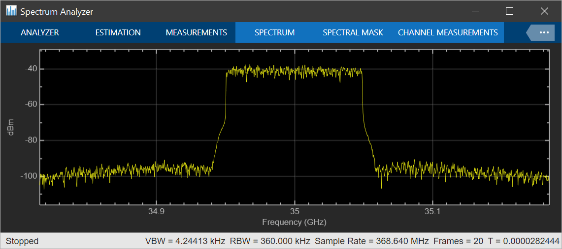
The time domain simulation is carried out in a new model that has the same structure as the previous model. However, the signal being transmitted is now an OFDM waveform, rather than a single tone signal. In addition, the received signal coming out of the RF Receiver is now measured using a spectrum analyzer and goes into a Baseband receiver subsystem that performs baseband demodulation and computes the EVM and MER of the received OFDM waveform.
model = 'simrfV2_TXRX_OFDM2';
open_system(model)
sim(model)
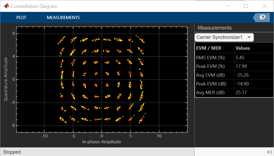
Part of the measured EVM can be attributed to distortion due to the frequency dependent antenna impedance and pattern. The Antenna block allows control over the modeling of these quantities via parameters in the Modeling pane of the Mask Parameters dialog box of the block:
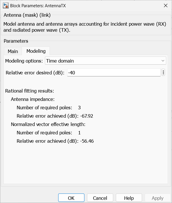
The choice of Time domain in the Modeling options creates an analytical rational model that approximates the antenna parameters within the entire frequency range of the simulation. The modeling choices for the Antenna block are similar to the modeling choices in other RF Blockset blocks such as the S-Parameter block. However, for the antenna block there are two separate quantities that require modeling: Antenna impedance and Normalized vector effective length. The modeling pane indicates the number of poles used and relative error achieved for each of those quantities.
bdclose(model)
clear model