Surrogate Optimization for Design of Digital Predistortion for Power Amplifier

Since R2024b

This example uses:

This example shows how to use surrogate optimization to automatically determine the coefficients of a digital predistortion (DPD) component to linearize an RF power amplifier (PA).

The DPD technique is used to correct for impairments of the PA by applying an inverse nonlinear operation on the input signal such that this inverse operation precompensates for the nonlinear response of the PA. The goal of DPD is to cumulatively achieve a linear amplification response, leading to overall improved transmission quality as quantified by standard system performance metrics such as error vector magnitude (EVM). The surrogate optimization approach presented in this example aims to efficiently automate the process of determining optimal coefficients or parameters of a DPD system to achieve this goal.

Here is an overview of the steps to perform the surrogate optimization procedure for the design of a DPD for an RF PA:

First, create an idealized baseband model of the RF system with DPD.
Second, define the optimization problem, and run the surrogate optimization algorithm.
Lastly, verify and validate the final DPD design.

Introduction

The introduction section of this example provides a background on fixed-coefficient digital predistortion and surrogate optimization.

Background on Fixed-Coefficient Digital Predistortion

In static or fixed-coefficient DPD architectures, the complex-valued coefficients of the DPD nonlinear operation are predetermined and fixed. In this case, the coefficients of a fixed predistorter can be optimized based on the following criteria:

A known, characterized RF PA. For example, the PA may be modeled by a memory polynomial or general memory polynomial, with or without cross terms, based on a specific complex-valued coefficient matrix.
Baseband and carrier waveforms adhering to a specific digital modulation scheme. For example, the carrier signal may be configured as per an orthogonal frequency-division multiplexing (OFDM) modulation scheme, and the baseband signal on each subcarrier may be encoded as per a quadrature amplitude modulation (QAM) scheme such as 64-QAM.
A performance metric to assess the linearization of the end-to-end system. For example, the optimization routine may seek to minimize the error between the output of the PA after predistortion and the expected output of the system without predistortion if the amplification were linear. Alternatively, the optimization routine may seek to minimize another quality metric such as the root mean squared (RMS) EVM.

This is in contrast to adaptive or dynamic DPD architectures, which use feedback loops and in-the-loop minimization routines to determine the DPD coefficients in real-time, aiming to achieve optimal linearization performance under varying operating conditions. In this approach, the algorithm adaptively adjusts the DPD coefficients to minimize an error metric that quantifies the deviation from linear performance or another heuristic that correlates with the same. For more information, see Adaptive DPD Design: A Top-Down Workflow.

Background on Surrogate Optimization

Surrogate optimization is a technique used to solve complex global optimization problems wherein direct evaluation of the objective function is computationally expensive or time-consuming. It is a well-established approach for design optimization tasks in which the objective function is evaluated using a black-box model, such as a Simulink® model.

Instead of evaluating the actual objective function at every iteration, the surrogate-based algorithm constructs and iteratively refines a simpler "surrogate model" that approximates the objective function, and it uses this surrogate to guide the search for optimal solutions. Because the surrogate is inexpensive to evaluate, the optimizer can use it to perform a large number of evaluations across a wide search space in a short amount of time, thereby reducing the computational burden that would be incurred if the optimizer were to evaluate the original objective function directly in search of a global optimum.

It is important to note that typical surrogate optimization implementations are intended for cases where the design variable space has finite, well-defined bounds. For more information, see Surrogate Optimization.

Idealized Baseband Model of RF System with DPD for 64-QAM OFDM Signal

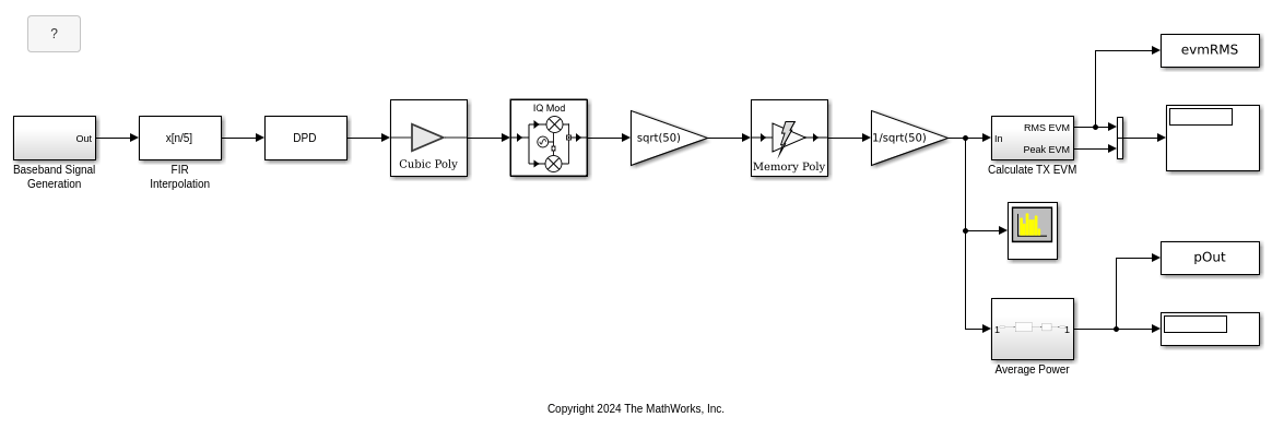
The top-level system consists of the following components:

Baseband Signal Generation — Generate a 64-QAM OFDM signal encoding a random sequence of integers ranging from 0 to 63.
FIR Interpolation — Upsample the signal and perform polyphase FIR interpolation to match the sample rate used for PA characterization.
DPD — Perform static predistortion using a memory polynomial structure built as per the fixed complex-valued coefficient matrix. The Coefficients block parameter specifies this coefficient matrix, and the Coefficient source parameter must be set to Property to enable it. In this example, the memory polynomial is of degree 3 and memory depth 3.
Amplifier and Mixer — Amplify and upconvert the signal to RF frequency. Note that the incoming signal is complex-valued, containing in-phase (I) and quadrature (Q) components, and so the complex baseband mixer is configured as an IQ modulator.
Power Amplifier — Perform power amplification on the RF signal consistent with the response characteristics of a narrowband, nonlinear power amplifier with memory effects. The PA model uses a memory polynomial with coefficients as specified in paModelMemPoly from PAcoefficientsComms.mat. Note that the Gain blocks before and after the Power Amplifier block serve to convert from power to voltage using the reference 50 Ω, as the memory polynomial model operates on voltage.
Calculate TX EVM — Model the receiver chain, which includes phase shift and gain compensation, downsampling the signal using polyphase FIR decimation, applying OFDM demodulation, visualizing the constellation of the received signal, and calculating the RMS EVM as a performance metric.
Spectrum Analyzer — Visualize the spectral response and adjacent channel power ratio (ACPR) of the output of the power amplifier.
Average Power — Measure the average output power of the system.

Open the top-level model.

model = "IdealizedPAWithStaticDPD";
open_system(model)

Note that this system is similar to those from the following examples:

The power amplifier model itself is based on the one obtained in Power Amplifier Characterization.

Store the block path to the DPD block to facilitate programmatic control of the DPD coefficient matrix.

blockDPD = model + "/DPD";

Also store the block paths of the scopes to facilitate visual assessment of the system performance and transmission quality with and without the DPD. In particular, store the block paths for the Spectrum Analyzer block in the top-level system and the Constellation Diagram block within the Calculate TX EVM subsystem.

blockSA = model + "/Spectrum Analyzer";
blockCD = model + "/Calculate TX EVM/Constellation Diagram";
close_system(blockSA)
close_system(blockCD)

Use `Simulink.SimulationInput` Object to Streamline Iterative Simulations

The optimization algorithm makes numerous calls to simulate the top-level model, each iteration corresponding to a different set of DPD coefficients. This means that each iteration requires a modification to specific block parameters prior to each simulation, namely a change to the DPD block's Coefficients parameter. The Simulink.SimulationInput object can be used to simplify this process of making temporary changes to the model and block parameters and the simulation variables, running multiple simulations across the parameter search space via the optimizer, and overall streamlining the programmatic control of iterative simulations.

Create a Simulink.SimulationInput object for this model.

simIn = Simulink.SimulationInput(model);

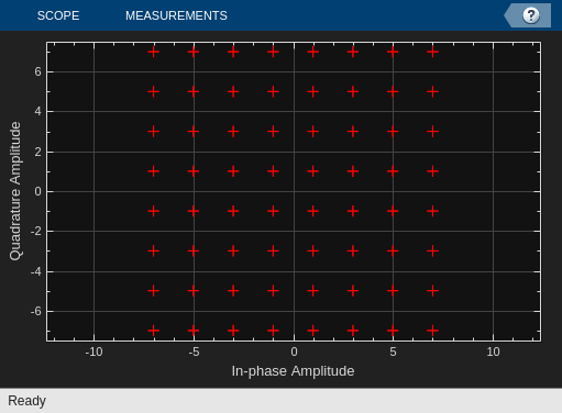
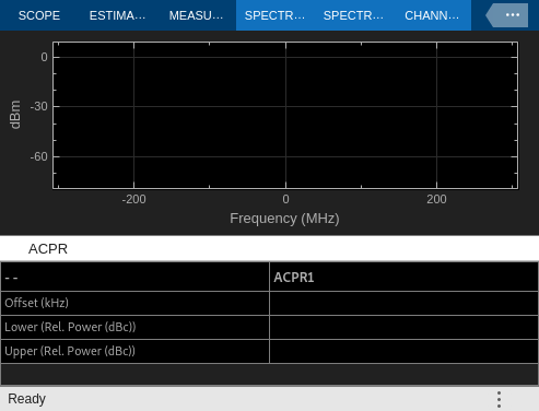
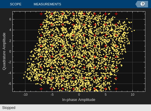
Simulate the model as is, where the DPD coefficient matrix yields no predistortion, such that the DPD is essentially a no-op. Observe that the PA's nonlinear impairments degrade the quality of the transmitted response, as seen in the constellation diagram and output spectrum, and as quantified by the RMS EVM of the last time step in the simulation.

coeffNoDPD = get_param(blockDPD,"Coefficients")
open_system(blockCD)
open_system(blockSA)
simOutNoDPD = sim(simIn)
evmRMSNoDPD = simOutNoDPD.evmRMS.Data(:,:,end)

coeffNoDPD =

    'complex([1 0 0; 0 0 0; 0 0 0])'


simOutNoDPD = 

  Simulink.SimulationOutput:
                 evmRMS: [1x1 timeseries] 
                   pOut: [1x1 timeseries] 

     SimulationMetadata: [1x1 Simulink.SimulationMetadata] 
           ErrorMessage: [0x0 char] 


evmRMSNoDPD =

   16.1032

Use Fast Restart to Accelerate Iterative Simulations

The optimization procedure entails many simulations of the model while each time modifying only the block parameters tied to the design variables to optimize. Sometimes, these design variables do not associate to a structural or topological change in the model or in its subsystems and blocks. In this case, multiple simulations may not require recompilation and termination of the model between each and every iteration. Especially for numerous iterative simulations, recompilation can be time-consuming and inefficient.

Fast Restart enables acceleration of iterative simulations by associating multiple instances of the simulation phase to a single instance of the compile phase, thereby avoiding time spent on recompilation and termination each time. Note that only some of the parameters are tunable between simulations when the model is initialized in Fast Restart. In this example, the DPD block's Coefficients parameter does support Fast Restart workflows. For more information, refer to the following pages:

Configure the model for Fast Restart using simIn.

simIn = setModelParameter(simIn,FastRestart="on");

Close both of the scopes prior to the optimization runs. This can help in improving simulation time.

close_system(blockCD)
close_system(blockSA)

High Level Overview of Optimization Problem Formulation

In this example, the goal of the optimization task is to determine the complex-valued coefficients of the DPD memory polynomial to minimize the RMS EVM of the demodulated received signal. This optimization problem can be formulated as follows:

The objective is to minimize the logarithm of the RMS EVM from the last time step of the simulation. Taking the logarithm here aids the numerical efficiency of the surrogate-based optimizer.
There are $2 \times M \times K$ parameters to optimize, where is the memory depth of the memory polynomial, and is the degree. The additional factor of 2 accounts for the real and imaginary parts of the complex-valued coefficients: $x_{mk}\mapsto\{\mathrm{Re}(x_{mk}),\mathrm{Im}(x_{mk})\}$ . Most of the Optimization Toolbox™ and Global Optimization Toolbox™ solvers do not directly handle complex-valued numbers, so the strategy here is to treat the real and imaginary parts as separate optimization variables. Collectively, the optimization vector is $x=\{x_{11r},x_{11i},...,x_{M1r},x_{M1i},...,x_{1Kr},x_{1Ki},...,x_{MKr},x_{MKi}\}$ , where and denote the real and imaginary parts, respectively.
The search space for each of the optimization parameters is bounded between –1.5 and +1.5. With the DPD disabled, the largest magnitude of the complex baseband input to the DPD block is on the order of 0.2, and that of the input to the PA block is on the order of 3. Accordingly, the bounds on the DPD coefficients are large enough to provide a wide search space but narrow enough to be practically and numerically stable.

Determine Optimal DPD Memory Polynomial Coefficients

Use the surrogateopt function to optimize the coefficients $x$ of the DPD memory polynomial to minimize the base 10 logarithm of the RMS EVM as per the high level overview of the problem formulation.

First specify the memory depth and degree of the memory polynomial.

M = 3;
K = 3;

Then specify the lower and upper bounds constraints from (3). These satisfy the inequalities $\rm{lb}3 \leq x \leq \rm{ub}3$ .

lb = -1.5*ones(1,2*M*K);
ub = 1.5*ones(1,2*M*K);

Configure the optimization search to begin with the coefficient matrix complex([1 0 0; 0 0 0; 0 0 0]), which maps to an initial optimization point [1 0 0 0 0 0 0 0 0 0 0 0 0 0 0 0 0 0]. This initial coefficient matrix corresponds to a system with no predistortion, which is a reasonable and natural starting point.

x0 = zeros(1,2*M*K);
x0(1,1) = 1;

To get reproducible results, reset the MATLAB® random number generator to its factory default settings

rng default

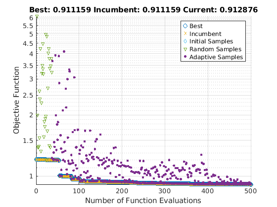
Run the surrogate optimization. The objective function, objFcn, is defined in Helper Functions. Optionally, set Verbose=true in the objective function call to print a log of the coefficient matrix and the RMS EVM for each optimization iteration that calls the objective function. For details on how to interpret the optimization plot results, see "Interpret surrogateoptplot" in the documentation for Global Optimization Toolbox.

[xOpt,fvalOpt,exitflag,output,trials] = surrogateopt( ...
    @(x)objFcn(x,simIn,blockDPD,M,K,Verbose=false),lb,ub, ...
    optimoptions("surrogateopt",InitialPoints=x0, ...
    MaxFunctionEvaluations=500,PlotFcn="surrogateoptplot"))

Set the y-axis of the optimization plot to logarithmic scaling to help closely examine the optimization trajectory.

yscale log

Verify and Validate Final DPD Design

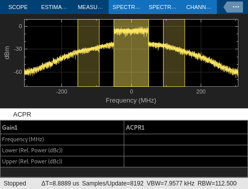
Simulate the model with the optimized DPD. Specifically, set the DPD block's coefficients to the optimal values obtained from the optimization results. Observe the improvement in the constellation diagram, output spectrum, and computed RMS EVM:

The constellation diagram shows a tighter clustering of points, indicating reduced distortion.
The output spectrum exhibits lower adjacent channel power, implying improved linearity.
The computed RMS EVM decreases, signifying enhanced signal quality.

This confirms the success of the DPD system design optimization and that the fixed-coefficient DPD can precompensate for the PA impairments to improve system linearization.

coeffOpt = reshape(complex(xOpt(1:2:end),xOpt(2:2:end)),M,K)
simIn = setBlockParameter(simIn,blockDPD,"Coefficients", ...
    "complex(" + mat2str(coeffOpt) + ")");
simIn = setModelParameter(simIn,FastRestart="off");
open_system(blockCD)
open_system(blockSA)
simOutOptimizedDPD = sim(simIn)
evmRMSOptimizedDPD = simOutOptimizedDPD.evmRMS.Data(:,:,end)

coeffOpt =

  -1.0340 + 0.3910i   1.5000 - 0.4280i  -0.8040 + 1.4661i
   0.0669 - 1.2973i  -0.1089 - 0.4513i   0.6207 - 0.3347i
  -0.1810 + 0.6829i   1.2627 + 0.1466i  -0.5141 + 0.6528i


simOutOptimizedDPD = 

  Simulink.SimulationOutput:
                 evmRMS: [1x1 timeseries] 
                   pOut: [1x1 timeseries] 

     SimulationMetadata: [1x1 Simulink.SimulationMetadata] 
           ErrorMessage: [0x0 char] 


evmRMSOptimizedDPD =

    8.1500

Verify that the output power of the system with the optimized DPD is similar to that of the system without DPD. This confirms that the improvement in EVM is not simply due to a scenario in which the DPD lowers the input power to cause the PA to operate in a back-off mode. This subtlety is important, because power back-off could lead to an artificially lowered EVM without addressing the underlying linearity issues. Checking for similar output power levels helps in validating the DPD design as one that genuinely enhances the linearity and performance of the PA without compromising on output power.

pOutNoDPD = simOutNoDPD.pOut.Data(:,:,end)
pOutOptimizedDPD = simOutOptimizedDPD.pOut.Data(:,:,end)

pOutNoDPD =

   40.2532


pOutOptimizedDPD =

   40.2675

Helper Functions

The following section defines the local, helper function used in this example to implement the simulation-based objective function.

function f = objFcn(x,simIn,blockDPD,M,K,options)
    arguments
        x
        simIn
        blockDPD
        M
        K
        options.Verbose (1,1) logical = false
    end

    persistent t
    if isempty(t)
        t = 0;
    end
    if options.Verbose
        tic
        disp("------------------------------------------------------")
    end


    coeff = reshape(complex(x(1:2:end),x(2:2:end)),M,K);
    if options.Verbose
        disp("Coefficients")
        disp(coeff)
    end
    simIn = setBlockParameter(simIn,blockDPD,"Coefficients", ...
        "complex(" + mat2str(coeff) + ")");

    simOut = sim(simIn);

    f = simOut.evmRMS.Data(:,:,end);
    if options.Verbose
        disp("RMS EVM = " + f)
    end
    f = log10(f);

    if options.Verbose
        t = t + toc;
        disp("Total elapsed time across all " + ...
            "objective function evaluations: " + t + " seconds.")
        disp("------------------------------------------------------")
    end
end

surrogateopt stopped because it exceeded the function evaluation limit set by 
'options.MaxFunctionEvaluations'.

xOpt =

  Columns 1 through 7

   -1.0340    0.3910    0.0669   -1.2973   -0.1810    0.6829    1.5000

  Columns 8 through 14

   -0.4280   -0.1089   -0.4513    1.2627    0.1466   -0.8040    1.4661

  Columns 15 through 18

    0.6207   -0.3347   -0.5141    0.6528


fvalOpt =

    0.9112


exitflag =

     0


output = 

  struct with fields:

        elapsedtime: 709.8296
          funccount: 500
    constrviolation: 0
               ineq: [1×0 double]
           rngstate: [1×1 struct]
            message: 'surrogateopt stopped because it exceeded the function evaluation limit set by ↵'options.MaxFunctionEvaluations'.'


trials = 

  struct with fields:

       X: [500×18 double]
    Fval: [500×1 double]