Lever Analysis

R2026b

Since R2026b

This example shows how to use the Simscape™ Lever (AB-PB) block to model lever systems in the position-based translational and angle-based rotational domains. Two models demonstrate the torque balance and kinematic constraints of a lever. The first model computes mechanical advantage from force measurements. The second model predicts which end of a lever contacts a wall when two forces act on it.

Question 1: What Is the Mechanical Advantage?

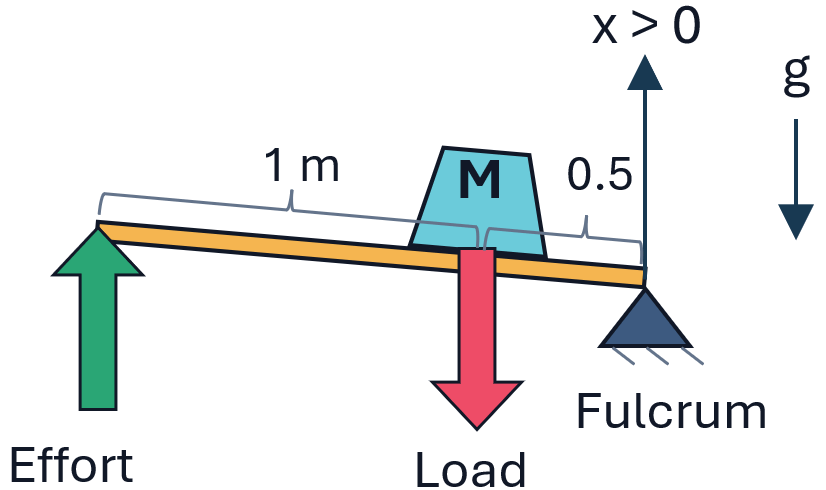
A second-class lever lifts a 10 kg mass against gravity. The fulcrum is fixed at the right end of the lever. The lever arm from the fulcrum to the load is 0.5 m and from the fulcrum to the effort is 1.5 m. A velocity source drives the effort end upward at 0.2 m/s. What is the mechanical advantage of this lever?

Analytical Solution

For an ideal lever, the mechanical advantage (MA) equals the ratio of the effort arm length to the load arm length:

$M A = \frac{L_{e f f o r t}}{L_{l o a d}} = \frac{1.5}{0.5} = 3$

From the torque balance about the fulcrum:

$L_{l o a d} F_{l o a d} + L_{e f f o r t} F_{e f f o r t} = 0$

The load force is the weight of the mass, acting downwards:

$F_{l o a d} = - m g = - 10 * 9.81 = - 98.1 N$

Solving for the effort force, acting upwards:

$F_{e f f o r t} = - \frac{L_{l o a d}}{L_{e f f o r t}} F_{l o a d} = - \frac{0.5}{1.5} \cdot (- 98.1) = 32.7 N$

The lever constrains the load velocity:

$v_{l o a d} = \frac{L_{l o a d}}{L_{e f f o r t}} v_{e f f o r t} = \frac{0.5}{1.5} v_{e f f o r t} = \frac{1}{3} v_{e f f o r t}$

The load travels in the same direction as the effort, but at one-third the speed. The displacement ratio is the inverse of the mechanical advantage.

Create variables with the calculated values:

loadForceCalculated = -98.1;  % [N]
effortForceCalculated = 32.7; % [N]
mechanicalAdvantageCalculated = abs(loadForceCalculated/effortForceCalculated);

Model

Open the model LeverMechanicalAdvantage.

open_system('LeverMechanicalAdvantage');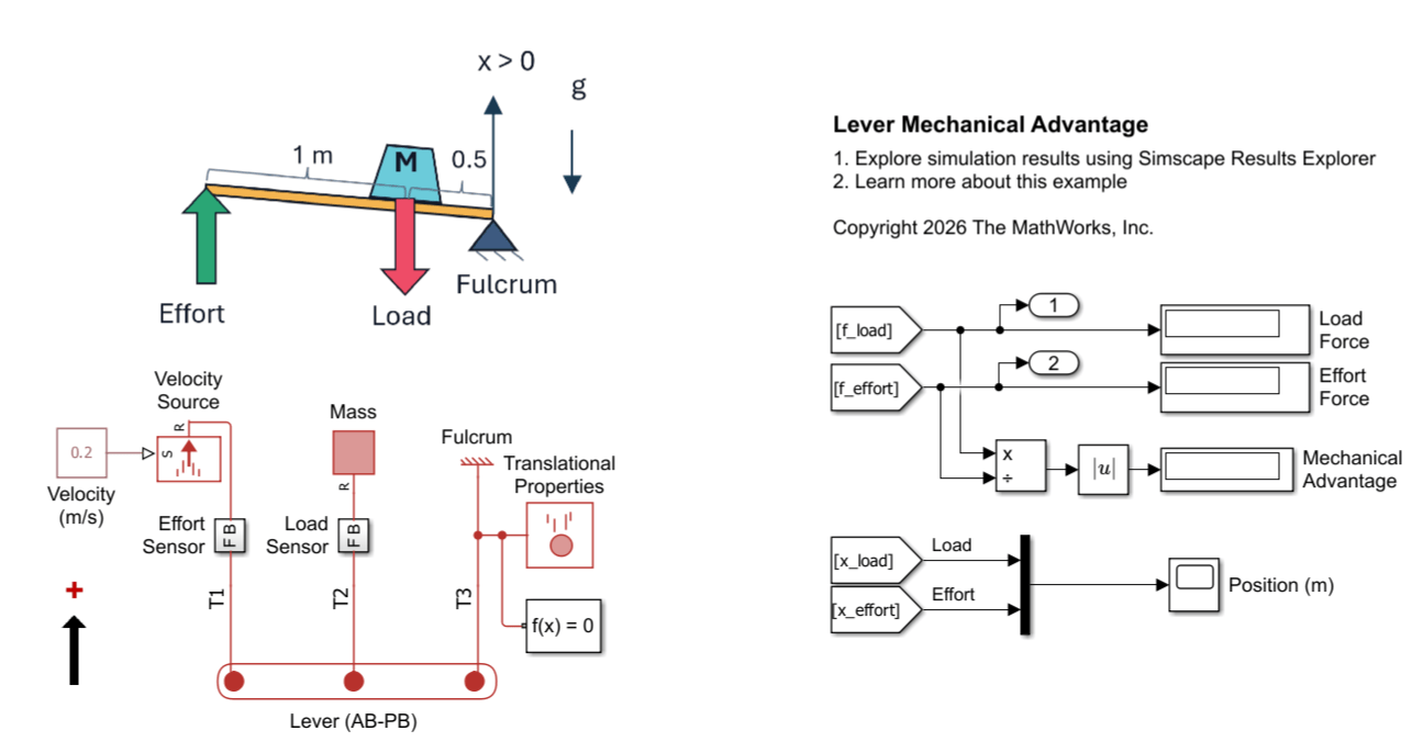

In this model the positive direction of the position-based translational network points upwards. The lever is placed perpendicular to the network's positive direction.

Sensors at the effort and load ports measure the port positions and forces. The force sensors measure force acting on the lever since the F ports are connected to the lever.

open_system('LeverMechanicalAdvantage/Effort Sensor');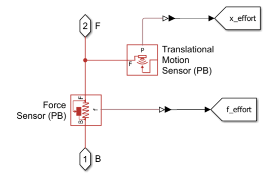

Simulation

Display blocks show the effort force, load force, and mechanical advantage. Outports save the final values of the effort and load forces in the Base Workspace.

sim('LeverMechanicalAdvantage');

Compare the simulated forces to the analytical solution. Forces are in units of N.

loadForceSimulated   = yout(end,1);
effortForceSimulated = yout(end,2);
mechanicalAdvantageSimulated = abs(loadForceSimulated/effortForceSimulated);

sprintf([ ...
    'Load force:           Calculated = %.2f N, Simulated = %.2f N\n' ...
    'Effort force:         Calculated = %.2f N, Simulated = %.2f N\n' ...
    'Mechanical advantage: Calculated = %.2f,   Simulated = %.2f'], ...
    loadForceCalculated, loadForceSimulated, ...
    effortForceCalculated, effortForceSimulated, ...
    mechanicalAdvantageCalculated, mechanicalAdvantageSimulated)

ans = 
    'Load force:           Calculated = -98.10 N, Simulated = -98.10 N
     Effort force:         Calculated = 32.70 N, Simulated = 32.70 N
     Mechanical advantage: Calculated = 3.00,   Simulated = 3.00'

Open the Position (m) scope and rerun the simulation.

open_system('LeverMechanicalAdvantage/Position (m)');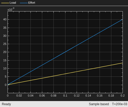

The Position (m) scope displays the effort and load positions versus time. The simulation shows that the load travels at 1/3 the velocity of the effort, matching the calculated response.

Question 2: Which End of the Lever Hits the Wall?

A 2 m vertical first-class lever is mounted 0.1 m from a wall. The fulcrum is 0.8 m from the top end and 1.2 m from the bottom end. Two horizontal forces push the lever ends away from the wall: 40 N at the top and 30 N at the bottom. This figure is a physical view of the system:

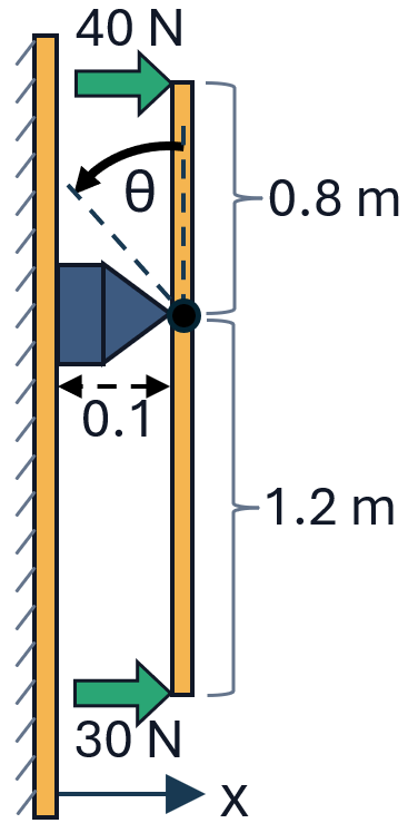
Which end of the lever contacts the wall?

Analytical Solution

Both forces try to push the lever end away from the wall, but they create opposing torques about the fulcrum. The torque from each force is:

$τ_{t o p} = {- L}_{t o p} F_{t o p} = - 0.8 * 40 = - 32 N m$

$τ_{b o t t o m} = L_{b o t t o m} F_{b o t t o m} = 1.2 * 30 = 36 N m$

The bottom force has a smaller magnitude but a longer moment arm, resulting in a larger torque compared to the top force. The net torque is:

$τ_{n e t} = τ_{b o t t o m} - τ_{t o p} = - 32 + 36 = 4 N m$

The net torque rotates the lever in the positive rotational direction, defined as counterclockwise in the physical view. Therefore, the top end moves towards the wall while the bottom end moves away from the wall.

Model

Open the model LeverRotation.

open_system('LeverRotation');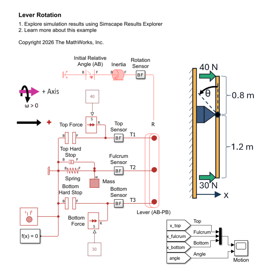

The model uses the Lever (AB-PB) block with its rotational port enabled. This port represents the rotational motion and inertia of the entire lever body. In this example, the rotational port is used to:

Set the initial lever angle to 0 deg with the Initial Relative Angle (AB) block.
Model the lever's rotational inertia about the fulcrum with the Inertia block.
Measure the lever angle with the Rotation Sensor subsystem.

The lever's Positive angle parameter is set to Corresponds to positive projected length. With this setting, a positive lever angle produces a positive projected length in the translational network. A projected length is the separation between two translational ports measured along the translational network direction. A positive projected length means that port T3 lies in the positive translational direction relative to port T1, while a negative projected length means that port T3 lies in the negative translational direction relative to port T1. Because the translational network in this model is horizontal and points to the right, a positive projected length means that port T3 is to the right of port T1, while a negative projected length means that port T3 is to the left of port T1.

When the lever angle is 0 deg, the lever is perpendicular to the translational network. In this state, all three ports occupy the same position in the horizontal translational network, and the ports have no separation in the translational network, so the projected lengths between T1, T2, and T3 are all zero. The Lever (AB-PB) block does not track the separation of ports in the direction perpendicular to the translational network (the vertical direction in this model).

The translational ports T1, T2, and T3 are generic translational conserving ports that can transmit any force or motion. None of the ports is inherently fixed or stationary. In this example, the fulcrum is modeled as a spring and damper that allow a small amount of translation of the pivot point. Translational Hard Stop blocks connected to ports T1 and T3 prevent either end of the lever from moving past a rigid wall at a position of 0 m.

Simulation

Open the Motion scope and simulate the model. The scope displays translational position of each lever port versus time (top subplot) and lever angle versus time (bottom subplot).

open_system('LeverRotation/Motion');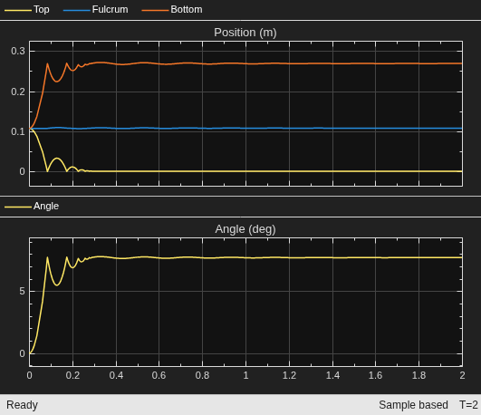

sim('LeverRotation');

The lever initially has an angle of 0 deg, so ports T1, T2, and T3 all occupy the same position in the translational network. This common position corresponds to the fulcrum location of about 0.1 m. As the simulation starts, the lever rotates in the positive (counterclockwise) direction about the fulcrum. The rotation causes the upper end of the lever to move in the negative translational direction (left) and the lower end to move in the positive translational direction (right). At approximately 0.1 sec, the upper end of the lever reaches the wall. The resulting impact causes several bounces before the motion dissipates and the lever comes to a rest.