Timelines and Execution Timing in Simulation
The Simulink® simulator simulates dynamic systems over time by computing the state and output values for the system of equations using time as the independent variable. The simulator computes the state and output values at discrete time points, called time steps, throughout the simulation. Often, models contain blocks and components that do not execute in every time step. For example, blocks that have a periodic sample time execute only at time steps that correspond to the specified sample time.
Understanding the timing and execution for different parts of a model can help you:
Post-process and validate data logged from simulation.
Debug and troubleshoot models and simulations.
Optimize the model for simulation performance.
Synchronize events in multi-rate and event-driven models.
Timelines
Timeline is a conceptual term that describes a collection of time steps that represents execution timing within the simulation. Execution timing relates to simulation time, which is the value of the time variable within the simulation. Simulation time is different from wall-clock time, which refers to elapsed time in the real world, such as the amount of time required to run a simulation.
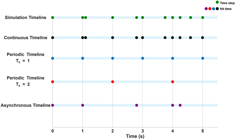
A simulation can contain multiple, overlapping timelines, with each timeline having its own set of hit times, which are the time steps that correspond to a given sample time. For example:
For a sample time of 1 second, the hit times are
0, 1, 2, ....For a sample time of 2 seconds, the hit times are
0, 2, 4,
                            ...
.
A timeline can be periodic, continuous, or asynchronous. The figure illustrates several common types of timelines that might arise from a model, including continuous, periodic, and asynchronous timelines. This list is not exhaustive but highlights representative timelines occurring during simulation.
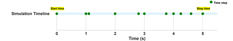
Simulation Timeline
The simulator determines time steps and hit times throughout the simulation based on the system dynamics, solver configuration, sample times, and execution semantics, such as events, defined in the simulated model. Changes to the model, the solver configuration, or the simulation configuration affect how the simulator determines time steps and hit times. Therefore, different simulations of the same model might produce simulation timelines with different time steps.
The simulation timeline contains all time steps taken in the simulation. Depending on the solver configuration and model dynamics, these time steps can be either fixed or variable. The first point in the simulation timeline corresponds to the simulation start time specified by the Start time model configuration parameter. The last point in the simulation timeline corresponds to the simulation stop time specified by the Stop time model configuration parameter.
Continuous Timeline
When a block has a continuous sample time, it produces a continuous signal. Blocks that have continuous sample time execute at every time step during the simulation. Numerical solvers approximate the evolution of the system states over time and determine the hit times that make up the continuous timeline.
The type of solver you choose for your model affects the continuous timeline in the simulation. When you use a variable-step solver, the hit times for continuous sample time can be irregularly spaced due to the solver varying the step size throughout the simulation.
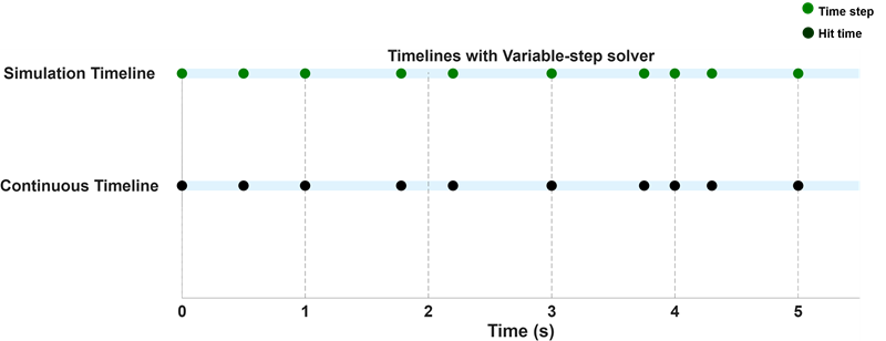
Choosing a fixed-step solver generates a continuous timeline with evenly spaced hit times defined by the fixed step size for the solver.
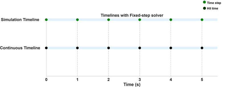
For more information on solvers, see Choose a Solver.
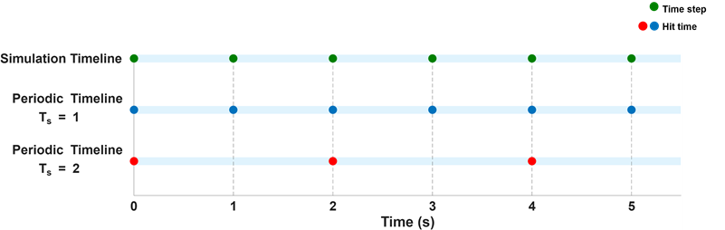
Periodic Timeline
When a timeline is periodic, hit times in the timeline occur at evenly spaced intervals. At each hit time, the simulator calculates the outputs of the blocks based on their inputs and current states. For more information, see Specify Sample Time.
The next image shows two periodic timelines, one with a sample time of 1 second and another with a sample time of 2 seconds. The simulation timeline includes the hit times of both periodic timelines.
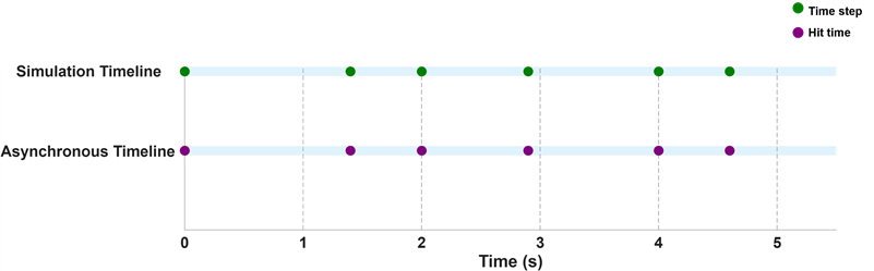
Asynchronous Timeline
Systems with events, function-call semantics, or aperiodic partitions can have asynchronous timelines. For more information on asynchronous sample times, see Types of Sample Time.
Suppose you have a model that uses a Function-Call Subsystem block. The top-level Inport block is configured to produce a function-call that executes at user-specified time points:
triggerTimes = [0, 1.4, 2, 2.9, 4, 4.6];
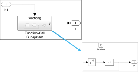
This image shows the corresponding asynchronous timeline and the simulation timeline.