命令行验证教程
此示例为可调速率限制器创建三个测试用例,并使用模型覆盖率工具的命令行 API 分析生成的模型覆盖率。
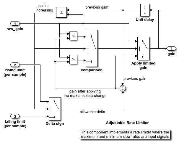
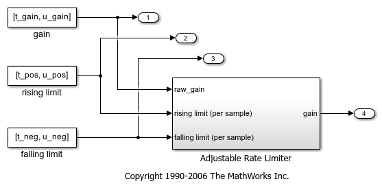
Simulink® 可调速率限制器模型
Simulink® 子系统可调速率限制器是模型“slvnvdemo_ratelim_harness”中的速率限制器。它使用三个 Switch 模块来控制何时限制输出以及应用的限制类型。
输入由 From Workspace 模块“增益”、“上升限制”和“下降限制”产生,它们生成分段线性信号。输入的值由 MATLAB® 工作区中定义的六个变量指定:t_gain、u_gain、t_pos、u_pos、t_neg 和 u_neg。
打开模型和可调速率限制器子系统。
modelName = 'slvnvdemo_ratelim_harness';
open_system(modelName);
open_system([modelName,'/Adjustable Rate Limiter']);
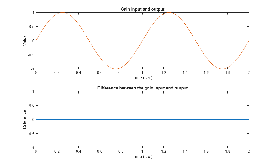
创建第一个测试用例
第一个测试用例验证当输入值没有快速变化时输出是否与输入匹配。它使用正弦波作为时变信号,并使用常数作为上升和下降限值。
t_gain = (0:0.02:2.0)';
u_gain = sin(2*pi*t_gain);
使用 MATLAB diff 函数计算时变输入的最小和最大变化。
max_change = max(diff(u_gain))
min_change = min(diff(u_gain))
max_change =

    0.1253


min_change =

   -0.1253
由于信号变化远小于 1 且远大于 -1,因此将速率限制设置为 1 和 -1。所有变量都存储在 MAT 文件“within_lim.mat”中,该文件在仿真之前加载。
t_pos = [0;2];
u_pos = [1;1];
t_neg = [0;2];
u_neg = [-1;-1];

save('within_lim.mat','t_gain','u_gain','t_pos','u_pos','t_neg','u_neg');
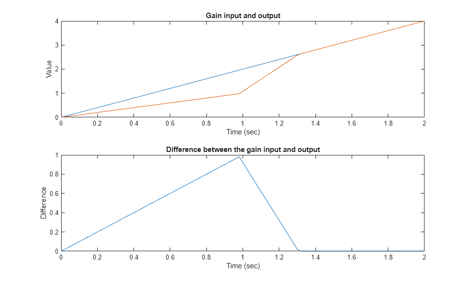
附加测试用例
第二个测试用例对第一个用例进行了补充,其增益上升超过了速率限制。一秒钟后,它会增加速率限制,以便增益变化低于该限制。
t_gain = [0;2];
u_gain = [0;4];
t_pos = [0;1;1;2];
u_pos = [1;1;5;5]*0.02;
t_neg = [0;2];
u_neg = [0;0];

save('rising_gain.mat','t_gain','u_gain','t_pos','u_pos','t_neg','u_neg');
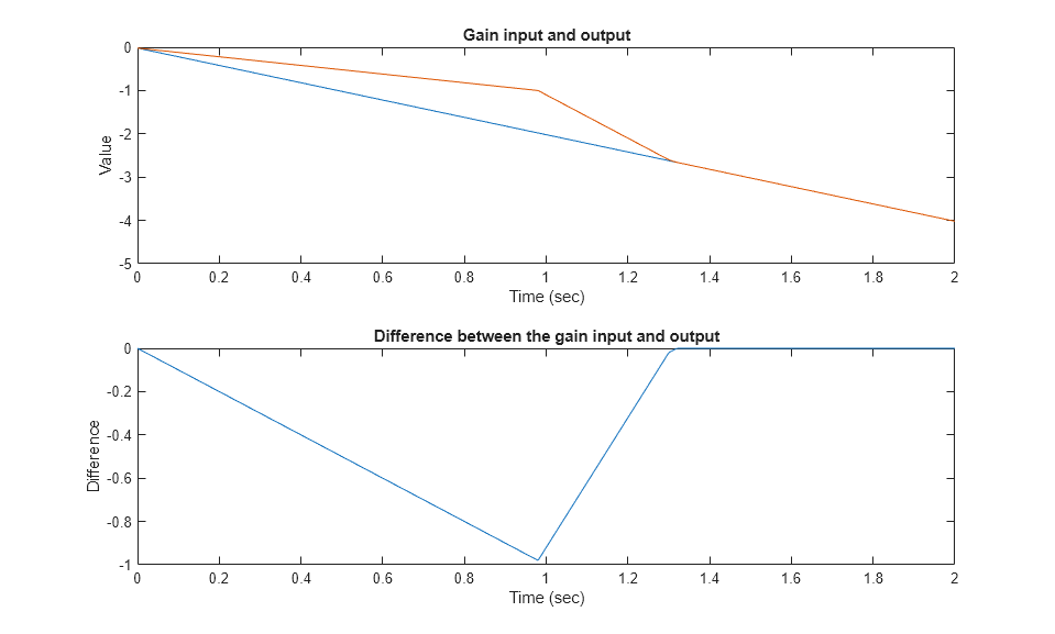
第三个测试用例是第二个测试用例的镜像,其中上升的增益被下降的增益所取代。
t_gain = [0;2];
u_gain = [-0.02;-4.02];
t_pos = [0;2];
u_pos = [0;0];
t_neg = [0;1;1;2];
u_neg = [-1;-1;-5;-5]*0.02;

save('falling_gain.mat','t_gain','u_gain','t_pos','u_pos','t_neg','u_neg');
定义覆盖率测试
测试用例使用 sim
在此示例中,使用仿真输入对象来设置覆盖率配置。
covSet = Simulink.SimulationInput(modelName);
covSet = setModelParameter(covSet,'CovEnable','on');
covSet = setModelParameter(covSet,'CovMetricStructuralLevel','Decision');
covSet = setModelParameter(covSet,'CovSaveSingleToWorkspaceVar','on');
covSet = setModelParameter(covSet,'CovScope','Subsystem');
covSet = setModelParameter(covSet,'CovPath','/Adjustable Rate Limiter');
covSet = setModelParameter(covSet,'StartTime','0.0');
covSet = setModelParameter(covSet,'StopTime','2.0');
执行覆盖率测试
加载第一个测试用例的数据,设置覆盖率变量名称,并使用 sim 执行模型。
load within_lim.mat
covSet = setModelParameter(covSet,'CovSaveName','dataObj1');
simOut1 = sim(covSet);
dataObj1
dataObj1 = ... cvdata
            version: (R2025b)
                 id: 1954
               type: TEST_DATA
               test: cvtest object
             rootID: 1956
           checksum: [1x1 struct]
          modelinfo: [1x1 struct]
          startTime: 12-Aug-2025 18:00:26
           stopTime: 12-Aug-2025 18:00:26
  intervalStartTime:
   intervalStopTime:
simulationStartTime: 0
 simulationStopTime: 2
             filter:
            simMode: Normal
通过检查输出是否与输入匹配来验证第一个测试用例。
subplot(211)
plot(simOut1.tout,simOut1.yout(:,1),simOut1.tout,simOut1.yout(:,4))
xlabel('Time (sec)'), ylabel('Value'),
title('Gain input and output');
subplot(212)
plot(simOut1.tout,simOut1.yout(:,1)-simOut1.yout(:,4))
xlabel('Time (sec)'),ylabel('Difference'),
title('Difference between the gain input and output');
以相同方式执行第二个测试用例并绘制结果。
请注意,一旦受限输出与输入出现偏差,它只能以最大斜率恢复。这就是为什么情节有一个不寻常的转折。一旦输入与输出匹配,两者就会一起改变。
load rising_gain.mat
covSet = setModelParameter(covSet,'CovSaveName','dataObj2');
simOut2 = sim(covSet);
dataObj2

subplot(211)
plot(simOut2.tout,simOut2.yout(:,1),simOut2.tout,simOut2.yout(:,4))
xlabel('Time (sec)'), ylabel('Value'),
title('Gain input and output');
subplot(212)
plot(simOut2.tout,simOut2.yout(:,1)-simOut2.yout(:,4))
xlabel('Time (sec)'), ylabel('Difference'),
title('Difference between the gain input and output');
dataObj2 = ... cvdata
            version: (R2025b)
                 id: 306
               type: TEST_DATA
               test: cvtest object
             rootID: 1956
           checksum: [1x1 struct]
          modelinfo: [1x1 struct]
          startTime: 12-Aug-2025 18:00:34
           stopTime: 12-Aug-2025 18:00:34
  intervalStartTime:
   intervalStopTime:
simulationStartTime: 0
 simulationStopTime: 2
             filter:
            simMode: Normal
执行第三个测试用例并绘制结果。
load falling_gain.mat
covSet = setModelParameter(covSet,'CovSaveName','dataObj3');
simOut3 = sim(covSet);
dataObj3

subplot(211)
plot(simOut3.tout,simOut3.yout(:,1),simOut3.tout,simOut3.yout(:,4))
xlabel('Time (sec)'), ylabel('Value'),
title('Gain input and output');
subplot(212)
plot(simOut3.tout,simOut3.yout(:,1)-simOut3.yout(:,4))
xlabel('Time (sec)'), ylabel('Difference'),
title('Difference between the gain input and output');
dataObj3 = ... cvdata
            version: (R2025b)
                 id: 428
               type: TEST_DATA
               test: cvtest object
             rootID: 1956
           checksum: [1x1 struct]
          modelinfo: [1x1 struct]
          startTime: 12-Aug-2025 18:00:36
           stopTime: 12-Aug-2025 18:00:36
  intervalStartTime:
   intervalStopTime:
simulationStartTime: 0
 simulationStopTime: 2
             filter:
            simMode: Normal
生成覆盖率报告
假设所有测试都已通过,则生成所有测试用例的综合报告以验证是否达到了 100% 的覆盖率。每个测试的覆盖率百分比显示在“模型层次结构”标题下。虽然单个测试都没有达到 100% 的覆盖率,但总体而言,它们实现了完全覆盖率。
cvhtml('combined_ratelim',dataObj1,dataObj2,dataObj3);
保存覆盖率数据
使用 cvsave 将收集的覆盖率数据保存在文件“ratelim_testdata.cvt”中。
cvsave('ratelim_testdata',dataObj1,dataObj2,dataObj3);
关闭模型并退出覆盖率环境
close_system('slvnvdemo_ratelim_harness',0);
clear dataObj*
加载覆盖率数据
打开模型后,使用 cvload 从文件“ratelim_testdata.cvt”恢复已保存的覆盖率测试。数据和测试在元胞数组中检索。
open_system('slvnvdemo_ratelim_harness');
[SavedTests,SavedData] = cvload('ratelim_testdata')
SavedTests =

  1×3 cell array

    {1×1 cvtest}    {1×1 cvtest}    {1×1 cvtest}


SavedData =

  1×3 cell array

    {1×1 cvdata}    {1×1 cvdata}    {1×1 cvdata}
操作覆盖率数据对象
使用重载运算符 +、- 和 * 操作 cvdata 对象。* 运算符用于查找两个覆盖率数据对象的交集,从而产生另一个 cvdata 对象。例如,以下命令生成所有三个测试的共同覆盖率的 HTML 报告。
common = SavedData{1} * SavedData{2} * SavedData{3}
cvhtml('intersection',common);
common = ... cvdata
            version: (R2025b)
                 id: 0
               type: DERIVED_DATA
               test: []
             rootID: 553
           checksum: [1x1 struct]
          modelinfo: [1x1 struct]
          startTime: 12-Aug-2025 18:00:26
           stopTime: 12-Aug-2025 18:00:36
  intervalStartTime:
   intervalStopTime:
             filter:
            simMode: Normal
从覆盖率数据对象中提取信息
使用 decisioninfo 从模块路径或模块句柄中检索决策覆盖率信息。输出是一个向量,分别包含单个模型对象的已实现结果和总体结果。
cov = decisioninfo(SavedData{1} + SavedData{2} + SavedData{3}, ...
                   'slvnvdemo_ratelim_harness/Adjustable Rate Limiter')
cov =

     6     6
使用检索到的覆盖率信息来访问百分比覆盖率。
percentCov = 100 * (cov(1)/cov(2))
percentCov = 100
当使用两个输出参量时,decisioninfo 返回一个结构体,该结构捕获 Simulink 模块或 Stateflow® 对象内的决策和结果。
[blockCov,desc] = decisioninfo(common, ...
         'slvnvdemo_ratelim_harness/Adjustable Rate Limiter/Delta sign')
descDecision = desc.decision
outcome1 = desc.decision.outcome(1)
outcome2 = desc.decision.outcome(2)
blockCov =

     0     2


desc =

  struct with fields:

           isFiltered: 0
    justifiedCoverage: 0
          isJustified: 0
      filterRationale: ''
             decision: [1×1 struct]


descDecision =

  struct with fields:

               text: 'Switch trigger'
    filterRationale: ''
         isFiltered: 0
        isJustified: 0
            outcome: [1×2 struct]


outcome1 =

  struct with fields:

               text: 'false (out = in3)'
     executionCount: 0
         executedIn: []
         isFiltered: 0
        isJustified: 0
    filterRationale: ''


outcome2 =

  struct with fields:

               text: 'true (out = in1)'
     executionCount: 0
         executedIn: []
         isFiltered: 0
        isJustified: 0
    filterRationale: ''