Compare Requirements and Design Variables Using Spider Plot
This example shows how to use a spider plot to compare requirement evaluations before and after optimizing the response. You can use a similar procedure to compare the values of sets of design variables.
Distillation Column Model
Open the distillation column model.
open_system('distillation_demo.slx')Open Response Optimizer
In the Simulink® model window, from the Apps tab, in the gallery, under Control Systems select Response Optimizer.
Alternatively, click the Response Optimization GUI with preloaded
data block in the model and skip the next step.
To load a preconfigured session, click the Response
Optimization tab. In the Open Session drop-down
list, select Open from model workspace. A window opens
where you select the Response Optimizer session to load. Select
distillation_optim and click OK.
The preconfigured step response requirements are loaded in the Response
Optimizer.
Evaluate Requirements Before Optimization
In the Response Optimization tab, click Evaluate Requirements.
A new variable, ReqValues, containing the evaluation of the
requirements appears in the Data area.
When optimizing the model response, you create a set of requirements that it must satisfy. If the requirements are violated, meaning that they evaluate to non-negative values, the design variables must be optimized. After the optimization, you can compare the original requirement value with the requirement evaluated using the optimized design variable values.
Plot Requirements Before Optimization
Plot the requirement value before optimization.
In the Data to Plot list, select
ReqValues.In the Add Plot list, select
Spider
                            plot
.
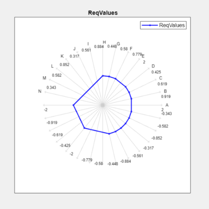
The plot has an axis for each edge-and-signal combination defined in the
distillation_demo/Desired Step Response check block. Points
on each axis represent the violation for that signal-edge combination and the plot
connects these points to form a closed polygon representing the initial design. Note
that some points are negative, representing satisfied constraints, and some
positive, representing violated constraints.
Optimize Model
To start the optimization, click Optimize.
A new variable, ReqValues1, containing the evaluation of the
requirements using the optimized design variables appears in the
Data area.
Compare Values Before and After Optimization
Compare the requirement values before and after optimization.
In the Data to Plot list, select
ReqValues1.In the Add Plot list, select
ReqValues.
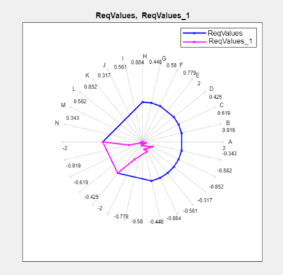
The optimized requirement values, ReqValues1, are all negative
or zero, indicating that all the constraints are satisfied.