Design Optimization with Uncertain Variables (Code)

Open Script

This example shows how to optimize a design when there are uncertain variables. You optimize the dimensions of a Continuously Stirred Tank Reactor (CSTR) to minimize product concentration variation and production cost in case of varying, or uncertain, feed stock.

Continuously Stirred Tank Reactor (CSTR) Model

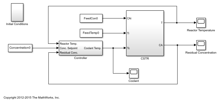
Continuously Stirred Tank Reactors (CSTRs) are common in the process industry. The Simulink® model, sdoCSTR, models a jacketed diabatic (i.e., non-adiabatic) tank reactor described in [1]. The CSTR is assumed to be perfectly mixed, with a single first-order exothermic and irreversible reaction, $A\rightarrow B$ . $A$ , the reactant, is converted to $B$ , the product.

In this example, you use the following two-state CSTR model, which uses basic accounting and energy conservation principles:

$\frac{d C_A}{dt} = \frac{F}{A * h}(C_{feed} - C_A)-r*C_A$

$\frac{d T}{dt} = \frac{F}{A * h}(T_{feed} - T) - \frac{H}{c_p \rho} r
-\frac{U}{c_p*\rho*h}(T - T_{cool})$

$r = k_0*e^{\frac{-E}{R*T}}$

, and $C_{feed}$ - Concentrations of A in the CSTR and in the feed [kgmol/m^3]

, $T_{feed}$ , and $T_{cool}$ - CSTR, feed, and coolant temperatures [K]

and $\rho$ - Volumetric flow rate [m^3/h] and the density of the material in the CSTR [1/m^3]

and - Height [m] and heated cross-sectional area [m^2] of the CSTR.

- Pre-exponential non-thermal factor for reaction $A\rightarrow B$ [1/h]

and - Activation energy and heat of reaction for $A\rightarrow B$ [kcal/kgmol]

- Boltzmann's gas constant [kcal/(kgmol * K)]

and - Heat capacity [kcal/K] and heat transfer coefficients [kcal/(m^2 * K * h)]

Open the Simulink model.

open_system('sdoCSTR');

The model includes a cascaded PID controller in the Controller subsystem. The controller regulates the reactor temperature, $T$ , and reactor residual concentration, $C_A$ .

CSTR Design Problem

Assume that the CSTR is cylindrical, with the coolant applied to the base of the cylinder. Tune the CSTR cross-sectional area, $A$ , and CSTR height, $h$ , to meet the following design goals:

Minimize the variation in residual concentration, . Variations in the residual concentration negatively affect the quality of the CSTR product. Minimizing the variations also improves CSTR profit.

Minimize the mean coolant temperature $T_{cool}$ . Heating or cooling the jacket coolant temperature is expensive. Minimizing the mean coolant temperature improves CSTR profit.

The design must allow for variations in the quality of supply feed concentration, $C_{feed}$ , and feed temperature, $T_{feed}$ . The CSTR is fed with feed from different suppliers. The quality of the feed differs from supplier to supplier and also varies within each supply batch.

Specify Design Variables

Select the following model parameters as design variables for optimization:

Cylinder cross-sectional area

Cylinder height

p = sdo.getParameterFromModel('sdoCSTR',{'A','h'});

Limit the cross-sectional area to a range of [1 2] m^2.

p(1).Minimum = 1;
p(1).Maximum = 2;

Limit the height to a range of [1 3] m.

p(2).Minimum = 1;
p(2).Maximum = 3;

Specify Uncertain Variables

Select the feed concentration and feed temperature as uncertain variables. You evaluate the design using different values of feed temperature and concentration.

pUnc = sdo.getParameterFromModel('sdoCSTR',{'FeedCon0','FeedTemp0'});

Create a parameter space for the uncertain variables. Use normal distributions for both variables. Specify the mean as the current parameter value. Specify a variance of 5% of the mean for the feed concentration and 1% of the mean for the temperature.

uSpace = sdo.ParameterSpace(pUnc);
uSpace = setDistribution(uSpace,'FeedCon0',makedist('normal',pUnc(1).Value,0.05*pUnc(1).Value));
uSpace = setDistribution(uSpace,'FeedTemp0',makedist('normal',pUnc(2).Value,0.01*pUnc(2).Value));

The feed concentration is inversely correlated with the feed temperature. Add this information to the parameter space.

%uSpace.RankCorrelation = [1 -0.6; -0.6 1];

The rank correlation matrix has a row and column for each parameter with the (i,j) entry specifying the correlation between the i and j parameters.

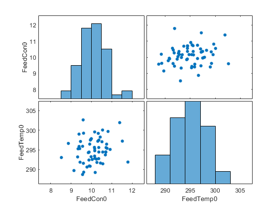
Sample the parameter space. The scatter plot shows the correlation between concentration and temperature.

rng('default'); %For reproducibility
uSmpl = sdo.sample(uSpace,60);
sdo.scatterPlot(uSmpl)

Ideally you want to evaluate the design for every combination of points in the design and uncertain spaces, which implies 30*60 = 1800 simulations. Each simulation takes around 0.5 sec. You can use parallel computing to speed up the evaluation. For this example you instead only use the samples that have maximum & minimum concentration and temperature values, reducing the evaluation time to around 1 min.

[~,iminC] = min(uSmpl.FeedCon0);
[~,imaxC] = max(uSmpl.FeedCon0);
[~,iminT] = min(uSmpl.FeedTemp0);
[~,imaxT] = max(uSmpl.FeedTemp0);
uSmpl = uSmpl(unique([iminC,imaxC,iminT,imaxT]) ,:);

Specify Design Requirements

The design requirements require logging model signals. During optimization, the model is simulated using the current value of the design variables. Logged signals are used to evaluate the design requirements.

Log the following signals:

CSTR concentration, available at the second output port of the sdoCSTR/CSTR block

Conc = Simulink.SimulationData.SignalLoggingInfo;
Conc.BlockPath               = 'sdoCSTR/CSTR';
Conc.OutputPortIndex         = 2;
Conc.LoggingInfo.NameMode    = 1;
Conc.LoggingInfo.LoggingName = 'Concentration';

Coolant temperature, available at the first output of the sdoCSTR/Controller block

Coolant = Simulink.SimulationData.SignalLoggingInfo;
Coolant.BlockPath               = 'sdoCSTR/Controller';
Coolant.OutputPortIndex         = 1;
Coolant.LoggingInfo.NameMode    = 1;
Coolant.LoggingInfo.LoggingName = 'Coolant';

Create and configure a simulation test object to log the required signals.

simulator = sdo.SimulationTest('sdoCSTR');
simulator.LoggingInfo.Signals = [Conc,Coolant];

Create Objective/Constraint Function

Create a function to evaluate the CSTR design. This function is called at each optimization iteration.

Use an anonymous function with one argument that calls the sdoCSTR_design function.

evalDesign = @(p) sdoCSTR_design(p,simulator,pUnc,uSmpl);

The evalDesign function:

Has one input argument that specifies the CSTR dimensions

Returns the optimization objective value

The sdoCSTR_design function uses a for loop that iterates through the sample values specified for the feed concentration. Within the loop, the function:

Simulates the model using the current iterate, feed concentration, and feed temperature values

Calculates the residual concentration variation and coolant temperature costs

To view the objective function, type edit sdoCSTR_design.

Evaluate Initial Design

Call the evalDesign function with the initial CSTR dimensions.

dInit = evalDesign(p)

dInit = 

  struct with fields:

              F: 10.9938
       costConc: 6.2936
    costCoolant: 4.7002

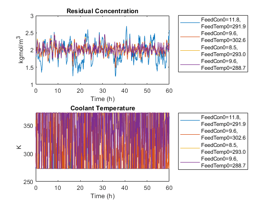
Plot the model response for the initial design. Simulate the model using the sample feed concentration values. The plot shows the variation in the residual concentration and coolant temperature.

sdoCSTR_plotModelResponse(p,simulator,pUnc,uSmpl);

The sdoCSTR_plotModelResponse function plots the model response. To view this function, type edit sdoCSTR_plotModelResponse.

Optimize Design

Pass the objective function and initial CSTR dimensions to sdo.optimize.

pOpt = sdo.optimize(evalDesign,p)

 Optimization started 2024-Sep-05, 19:03:04

                               max                     First-order 
 Iter F-count        f(x)   constraint    Step-size    optimality
    0      4       5.0414            0
    1      8      2.47564            0         2.01        0.606
    2     16      2.44299            0        0.124        0.857
    3     21      2.44108            0        0.051       0.0634
    4     22      2.44108            0      0.00076       0.0179
Local minimum possible. Constraints satisfied.

fmincon stopped because the size of the current step is less than
the value of the step size tolerance and constraints are 
satisfied to within the value of the constraint tolerance.
 
pOpt(1,1) =
 
       Name: 'A'
      Value: 2
    Minimum: 1
    Maximum: 2
       Free: 1
      Scale: 0.5000
       Info: [1x1 struct]

 
pOpt(2,1) =
 
       Name: 'h'
      Value: 2.3325
    Minimum: 1
    Maximum: 3
       Free: 1
      Scale: 2
       Info: [1x1 struct]

 
2x1 param.Continuous

Evaluate Optimized Design

Call the evalDesign function with the optimized CSTR dimensions.

dFinal = evalDesign(pOpt)

dFinal = 

  struct with fields:

              F: 2.4411
       costConc: 1.4571
    costCoolant: 0.9840

Plot the model response for the optimized design. Simulate the model using the sample feed concentration values. The optimized design reduces the residual concentration variation and average coolant temperature for different feed stocks.

sdoCSTR_plotModelResponse(pOpt,simulator,pUnc,uSmpl);

Related Examples

To learn how to use sensitivity analysis to explore the CSTR design space and select an initial design for optimization, see Design Exploration Using Parameter Sampling (Code).

References

[1] Bequette, B.W. Process Dynamics: Modeling, Analysis and Simulation. 1st ed. Upper Saddle River, NJ: Prentice Hall, 1998.

% Close the model
bdclose('sdoCSTR')