Estimate Model Parameter Values (GUI)

Engine Throttle System Model

Open the Simulink® model.

open_system('spe_engine_throttle')

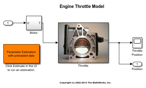
Throttle Model Description

The throttle controls the air mass flow into the intake manifold of an engine. The throttle body contains a butterfly valve that opens when the driver presses down on the accelerator pedal. This lets more air enter the cylinders and causes the engine to produce more torque.

A DC motor controls the opening angle of the butterfly valve. There is also a spring attached to the valve to return it to its closed position when the DC motor is de-energized. The amount of rotation of the valve is limited to approximately 90 degrees. Therefore, if a large command input is applied to the motor, the valve hits the hard stops preventing it from rotating further.

The motor is modeled as a torque gain and a time-delay input with parameters Kt and input_delay. The butterfly valve is modeled as a mass-spring-damper system with parameters J, c and k. This system is augmented with hard stops to limit the valve opening to 90 degrees. The model components are known, however, the parameter values of the system are not known accurately.

Estimation Experiment Data

Double-click the Parameter Estimation with preloaded data block in the model to open a pre-configured estimation GUI session.

The saved estimation project defines three experiments; the EstimationData experiment is used for parameter estimation, while ValidationData1, ValidationData2 are used for validating the estimated parameters. The EstimateData experiment is plotted.

The signal data for the experiments can be imported from various sources including MATLAB® variables, MAT files, Excel® files, or comma-separated-value files. See Importing and Preprocessing Experiment Data (GUI) for more information.

The experiment plot is also used to see how well the measured data matches the current model. Click Plot Model Response to display simulated signal data on the experiment plots.

The simulation results show that the model does not match the measured data and that model parameters need to be estimated.

Estimated Parameters

The next step is to define the parameter to estimate. Click Select Parameters to open a dialog box to select model parameters to estimate. This example contains four unknown parameters; the butterfly valve inertia, J; the damping coefficient, c; the return spring constant, k; the time lag in motor response, input_delay.

Since it is known from physical insight that all of these parameters have positive values, set their lower limits to zero. Also, put an upper bound of 0.1 sec on the input_delay parameter. You can also select an initial value for the parameters. These can come from some quick calculations of some formulas that determine the parameters.

The Estimation Task

After selecting the parameters for estimation, select the experiments to use for estimation. Click Select Experiments and select EstimationData for estimation.

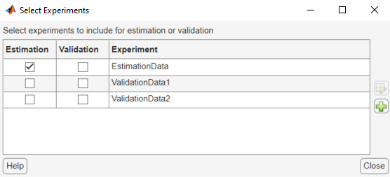
You can now start the estimation but first create plots to monitor the estimation progress. Click Add Plot and select Parameter Trajectory. This creates a plot that shows how the estimated parameter values change during estimation. Click the arrow at the right-hand side of the plot tab and choose Tile All... > Left/Right to layout the plots so that Experiment plot:EstimationData and EstimatedParams are both visible.

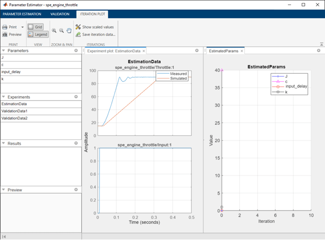
Click the Estimate button to start the estimation. You can modify estimation options by setting the Cost Function combobox and clicking More Options.

While the estimation is running, the plots update and a dialog box showing estimation progress appears. The progress dialog box shows the estimation iterations, the number of times the model has been evaluated (F-count), and the estimation cost at each iteration.

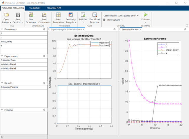
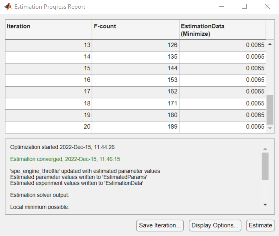
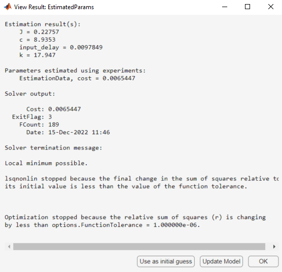
After a number of iterations the estimation converges and terminates. The model is updated with the estimated parameters and the estimation results are saved in the data browser. To see the details of the estimation result, right-click EstimatedParams and select Open.

Validation

It is important to validate the estimation results against other experiments. A successful estimation will not only match the experimental data that was used for estimation but also other independent measured data that were collected in experiments.

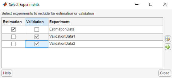
To select experiments for validation, click the Validation tab and click Select Experiments. Select both ValidationData1 and ValidationData2 for validation.

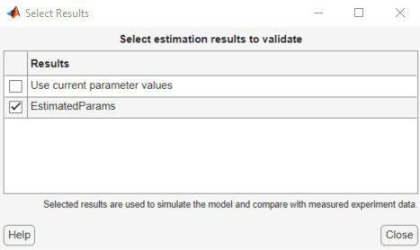
Click Select Results to Validate to select the estimation results to use for validation. Select EstimatedParams and clear Use current parameter values.

Click Validate to validate the estimation result against the validation experiments. Validation simulates the model using the estimated parameters and selected experiments and creates plots showing the measured and simulation data. Drag the Experiment plot:ValidationData1 plot tab to the left so that the Experiment plot:ValidationData1 and Experiment plot:ValidationData2 are both visible.

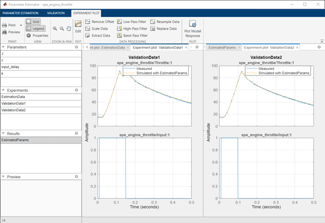
The validation plots confirm that the estimation was successful. The plots also show that the estimated parameters are robust enough to handle a variety of inputs.

Related Examples

To learn how to estimate model parameters using the sdo.optimize command, see Estimate Model Parameter Values (Code).