Design Optimization for Robustness to Model Component Tolerances
This example shows how to use the Sensitivity Analyzer and Response Optimizer apps to optimize design variables so that a model satisfies design requirements, even in the presence of uncertainties in the model parameters.
The model is of a single-ended primary-inductor converter (SEPIC) circuit used as a DC-DC converter to control a string of LEDs. The converter uses a switch to control the supplied voltage and is can output a higher voltage than the source voltage. It is similar to a buck-boost converter, but without polarity inversion. This circuit contains several electrical components, each of which has a nominal value and a tolerance. For more information, see SEPIC Voltage Control (Simscape Electrical).
The goal is to tune the PI controller of the circuit such that the response of the circuit satisfies the requirements even when considering variations of the circuit component in the range of the tolerance for each component.
mdlName = 'sdoSEPICController';
open_system(mdlName);
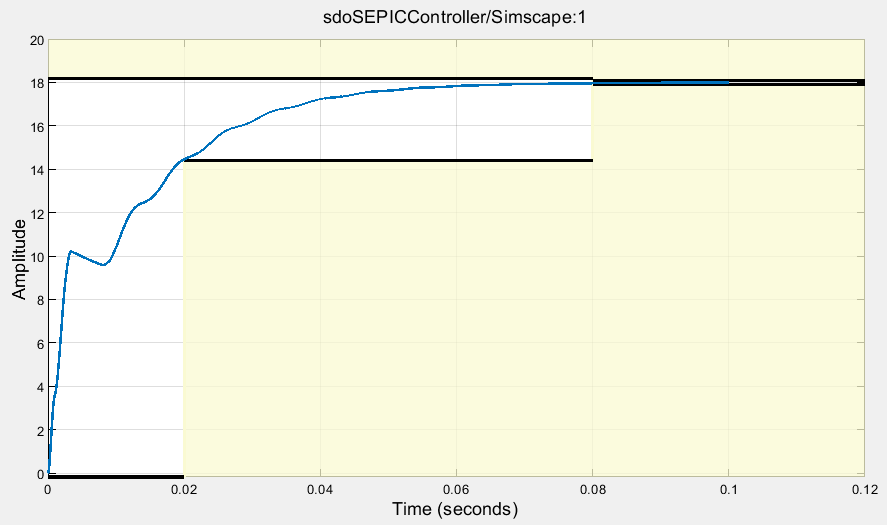
The design requirement is that the step response of the model output has the following characteristics.
Final output of 18 V
Rise time of 0.02 s
Settling time of 0.08 s
Percent overshoot no greater than 1%
Setting percentage no greater than 0.5%
The controller gains are an integral gain, Ki, of 3 and a proportional gain, Kp, of 0.03. Assuming nominal values for the circuit components, the system response with these gains satisfies the step-response requirements.
In addition to the load resistor, the SEPIC circuit has seven components to consider. The nominal circuit values, tolerances, and corresponding minimum and maximum values are shown in the following table.
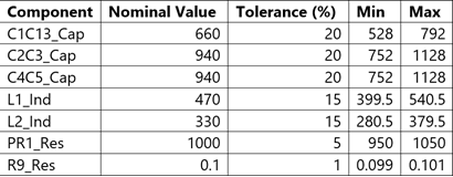
In addition to these circuit components, the load resistance for the circuit will be varied between 50 and 350 Ω.
Set Up Model for Sensitivity Analysis
To analyze how the model is affected by uncertainties in the model parameters, use the Sensitivity Analyzer app.
ssatool(mdlName)
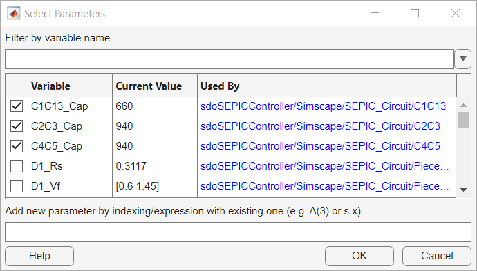
In the app, select the parameters to vary and analyze their effect on the requirements. To do so, click Select Parameters and create a new parameter set. Select the variables of interest, C1C13_Cap, C2C3_Cap, C4C5_Cap, L1_Ind, L2_Ind, PR1_Res, R9_Res and Rload_Res.
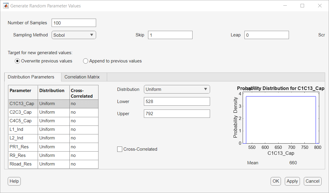
Next, specify how to generate values for these parameters. Click Generate Values and then Generate Random Values. Set the number of samples to 100 and set Sampling Method to Sobol. Specify the lower and upper bounds for each variable as specified in the table above. For Rload_Res, set the lower bound to 50 and the upper bound to 350. Click OK generate the sample values.
Finally, define the design requirements. From the toolstrip, click New Requirement and then Step Response Envelope. In the Create Requirement dialog box, enter the desired step-response characteristics.
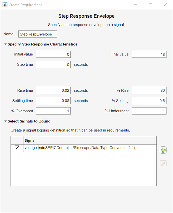
To specify which signal the step response requirement applies to, click ![]() near the bottom of the dialog box. In the model, click the output of the system,
near the bottom of the dialog box. In the model, click the output of the system, voltSEPIC.

This signal is added to the Create Signal Set dialog box. In that dialog box, click OK, and click OK in the Step Response Envelope dialog box.

For convenience, the setup described up to this point is saved in a file. The following commands launch the Sensitivity Analyzer app preconfigured with this setup:
load sdoSEPICController_sasessionSetup.mat
ssatool(SDOSessionData);
Evaluate the Model
Now that you have specified parameter samples and design requirements have been specified, evaluate the model to determine if each parameter sample satisfies the requirement. In the app, click Evaluate Model to simulate the model with 100 randomly sampled values for the eight parameters.
load sdoSEPICController_sasessionInitial.mat
ssatool(SDOSessionData);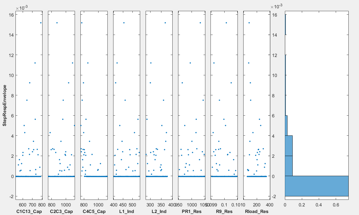
The majority of the parameter values tested satisfy the requirements, as indicated by a zero or negative StepRespEnvelope value. However, there are some sets of parameter values tested which do not satisfy the requirements, indicated by a positive evaluation value. The controller gains should be tuned further to account for these parameter variations. Performing a full optimization which accounts for all 8 uncertain variables would take a considerable amount of time. Just considering the minimum and maximum values for each parameter would require 256 model evaluations to test every combination. Instead, Sensitivity Analyzer can be used to identify the parameters which are most influential on the requirements being satisfied.
In the Statistics tab in Sensitivity Analyzer, select Correlation and Standardized Regression for methods and Linear and Ranked for types. Click on Compute Statistics.

From the results, the C4C5_Cap parameter is the most influential followed by Rload_Res. The C4C5 capacitor maintains the voltage for the load, so it is expected to be the most influential component. The load resistance is the next most influential characteristic of the overall system.
Optimize Response with Uncertain Variables
In the Sensitivity Analysis tab, select Optimize > Create Response Optimization Session. Select the step response envelope requirement and click OK to create a response optimizer session.
Add the design variables by clicking on the drop-down next to Design Variables Set and selecting New. Select the PI gain parameters, Kp and Ki and add them as design variables using the arrow in the middle.
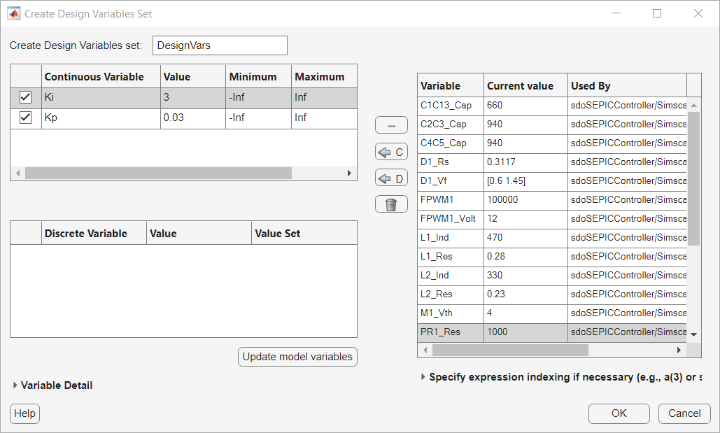
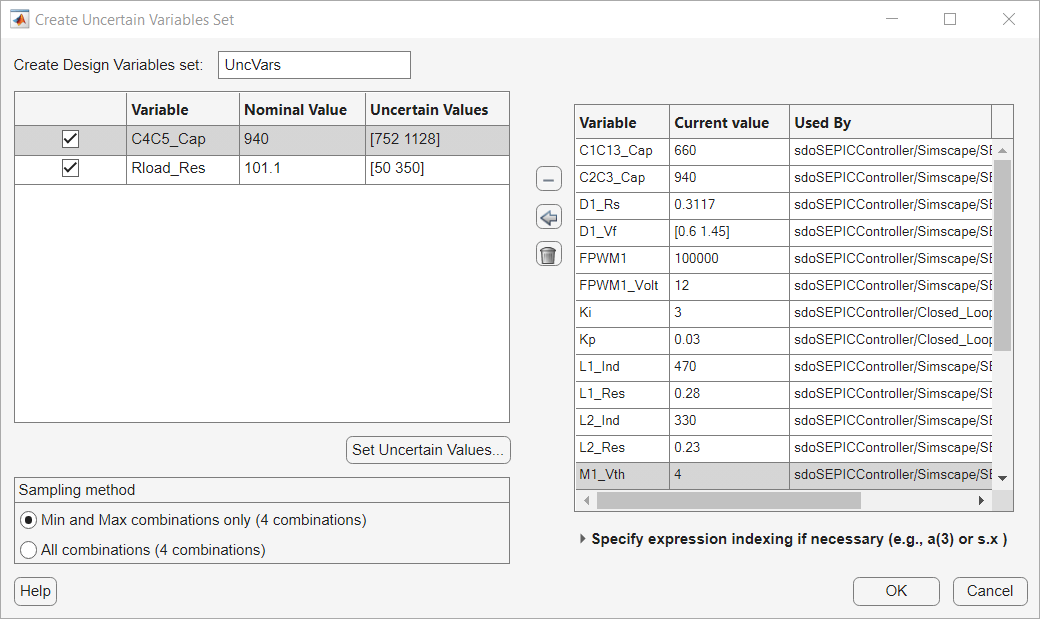
Click OK to save the design variable set. Follow the same steps to add an Uncertain Variable Set. The only variables that will be considered for the optimization are C4C5_Cap and Rload_Res. Define the minimum and maximum values for these parameters. Each function evaluation during optimization will then only require 5 model evaluations: 1 for the nominal values, and 4 for each combination of minimum and maximum uncertain variable values.
For this problem, a pattern search method is useful, due to the problem being nonsmooth. Select Options > Optimization Options change the Method to Pattern search.
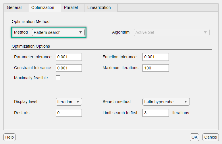
Click OK to save the options. Then, click Optimize to optimize the controller gains while considering the uncertain variables.
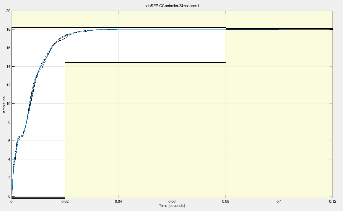
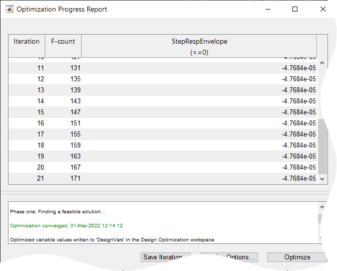
The optimization algorithm converged to values of Kp and Ki which satisfy the requirements when considering the minimum and maximum values for the 2 parameters identified to be the most influential.
load sdoSEPICController_sdosession.matWarning: While loading an object of class 'optim.options.PatternsearchOptions': Unrecognized method, property, or field 'TolFunValue' for class 'optim.options.PatternsearchOptions'.
sdotool(SDOSessionData)
Perform Final Sensitivity Analysis
Another sensitivity analysis should be performed to determine if the gain values found during optimization are robust to the parameter value uncertainties. In addition to the 100 random points tested previously, every combination of minimum and maximum value for the 8 parameters will also be tested. From the Generate Values drop-down, select Generate Gridded Values. Set the minimum and maximum values for each of the 8 parameters and click on Append to add these combinations to the set of parameter values tested.
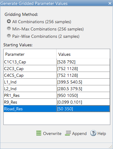
Evaluate the model again using this new set of parameter values.
load sdoSEPICController_sasessionFinal.mat
ssatool(SDOSessionData)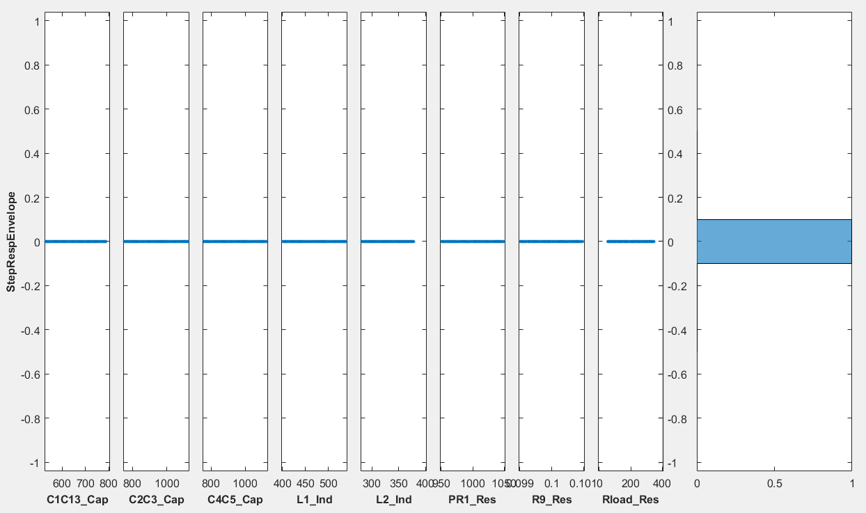
The new set of optimized gains satisfy the requirements for all 356 sets of parameter values tested.
Summary
By using both the Sensitivity Analyzer and Response Optimizer apps, the gains of the controller were optimized to be robust to uncertainties in the parameter values. Performing just a response optimization for the model would require a significant number of model evaluations for each iteration if all of the uncertain variables were considered. Each function evaluation for the optimization would require 257 model evaluations when considering just the minimum and maximum values for all 8 uncertain variables. Using Sensitivity Analyzer, the parameters affecting the performance most significantly could be identified and used for response optimization. This drastically cut down on the number of model evaluations. A table showing the number of model evaluations for the whole process is shown below.

Performing a response optimization with all 8 uncertain variables considered took 6168 model evaluations. This is more than 4 times as many evaluations than the method showcased.
The final gains found were Ki = 4.4947 and Kp = 0.0198; about a 50 percent difference from the original values. To see how variations in the design variables affect the requirements, sensitivity analysis can also be performed on the tuned gains, Kp and Ki. In Sensitivity Analyzer, create a new parameter set which includes Kp and Ki. Generate 100 uniformly random points and evaluate the model.
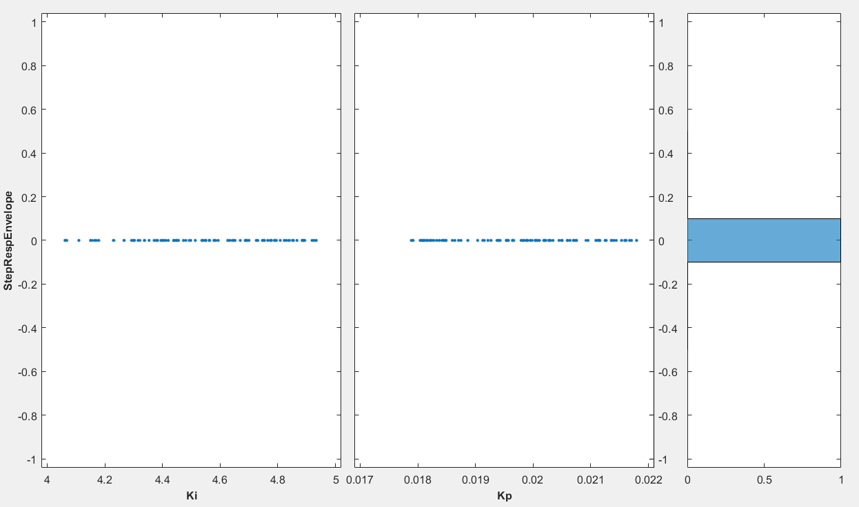
The system is also robust to variations in the controller gains; at least for the nominal component values.
Alternative Methods of Optimization
The results from performing response optimization with all 8 uncertain variables considered during optimization are shown below. These results used gradient descent as the optimization method instead of pattern search and required 6168 model evaluations.
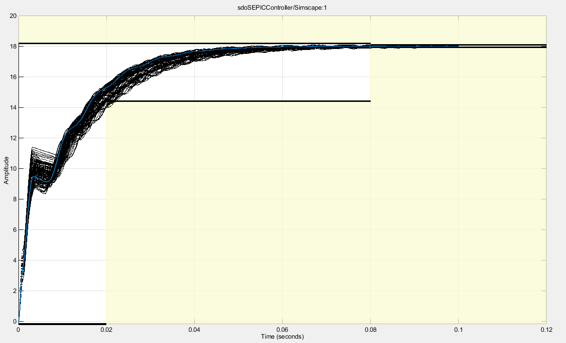
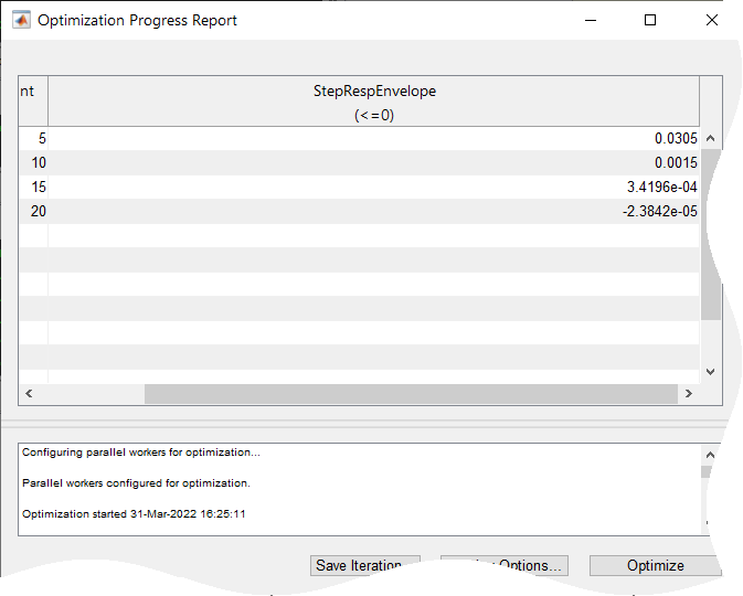
While the gradient descent optimization took fewer iterations and function evaluations to converge to a feasible solution, all 8 uncertain variables needed to be considered for it to be successful. This is due to the nonsmooth nature of the problem. While gradient descent is able to make progress with a subset of the uncertain variables, the solution is not robust when considering all uncertain variables.