Analyze Stock Prices Using Factor Analysis

Factor Loadings

Load the sample data.

load stockreturns

Suppose that over the course of 100 weeks, the percent change in stock prices for ten companies has been recorded. Of the ten companies, the first four can be classified as primarily technology, the next three as financial, and the last three as retail. It seems reasonable that the stock prices for companies that are in the same sector might vary together as economic conditions change. Factor analysis can provide quantitative evidence.

First specify a model fit with three common factors. By default, factoran computes rotated estimates of the loadings to try and make their interpretation simpler. But in this example, specify an unrotated solution.

[Loadings,specificVar,T,stats] = factoran(stocks,3,'rotate','none');

The first two factoran output arguments are the estimated loadings and the estimated specific variances. Each row of the loadings matrix represents one of the ten stocks, and each column corresponds to a common factor. With unrotated estimates, interpretation of the factors in this fit is difficult because most of the stocks contain fairly large coefficients for two or more factors.

Loadings

Loadings = 10×3

    0.8885    0.2367   -0.2354
    0.7126    0.3862    0.0034
    0.3351    0.2784   -0.0211
    0.3088    0.1113   -0.1905
    0.6277   -0.6643    0.1478
    0.4726   -0.6383    0.0133
    0.1133   -0.5416    0.0322
    0.6403    0.1669    0.4960
    0.2363    0.5293    0.5770
    0.1105    0.1680    0.5524

Factor rotation helps to simplify the structure in the Loadings matrix, to make it easier to assign meaningful interpretations to the factors.

From the estimated specific variances, you can see that the model indicates that a particular stock price varies quite a lot beyond the variation due to the common factors. Display estimated specific variances.

specificVar

specificVar = 10×1

    0.0991
    0.3431
    0.8097
    0.8559
    0.1429
    0.3691
    0.6928
    0.3162
    0.3311
    0.6544

A specific variance of 1 would indicate that there is no common factor component in that variable, while a specific variance of 0 would indicate that the variable is entirely determined by common factors. These data seem to fall somewhere in between.

Display the p-value.

stats.p

ans = 
0.8144

The p-value returned in the stats structure fails to reject the null hypothesis of three common factors, suggesting that this model provides a satisfactory explanation of the covariation in these data.

Fit a model with two common factors to determine whether fewer than three factors can provide an acceptable fit.

[Loadings2,specificVar2,T2,stats2] = factoran(stocks, 2,'rotate','none');

Display the p-value.

stats2.p

ans = 
3.5610e-06

The p-value for this second fit is highly significant, and rejects the hypothesis of two factors, indicating that the simpler model is not sufficient to explain the pattern in these data.

Factor Rotation

As the results illustrate, the estimated loadings from an unrotated factor analysis fit can have a complicated structure. The goal of factor rotation is to find a parameterization in which each variable has only a small number of large loadings. That is, each variable is affected by a small number of factors, preferably only one. This can often make it easier to interpret what the factors represent.

If you think of each row of the loadings matrix as coordinates of a point in M-dimensional space, then each factor corresponds to a coordinate axis. Factor rotation is equivalent to rotating those axes and computing new loadings in the rotated coordinate system. There are various ways to do this. Some methods leave the axes orthogonal, while others are oblique methods that change the angles between them. For this example, you can rotate the estimated loadings by using the promax criterion, a common oblique method.

[LoadingsPM,specVarPM] = factoran(stocks,3,'rotate','promax');
LoadingsPM

LoadingsPM = 10×3

    0.9452    0.1214   -0.0617
    0.7064   -0.0178    0.2058
    0.3885   -0.0994    0.0975
    0.4162   -0.0148   -0.1298
    0.1021    0.9019    0.0768
    0.0873    0.7709   -0.0821
   -0.1616    0.5320   -0.0888
    0.2169    0.2844    0.6635
    0.0016   -0.1881    0.7849
   -0.2289    0.0636    0.6475

Promax rotation creates a simpler structure in the loadings, one in which most of the stocks have a large loading on only one factor. To see this structure more clearly, you can use the biplot function to plot each stock using its factor loadings as coordinates.

biplot(LoadingsPM,'varlabels',num2str((1:10)'));
axis square
view(155,27);

This plot shows that promax has rotated the factor loadings to a simpler structure. Each stock depends primarily on only one factor, and it is possible to describe each factor in terms of the stocks that it affects. Based on which companies are near which axes, you could reasonably conclude that the first factor axis represents the financial sector, the second retail, and the third technology. The original conjecture, that stocks vary primarily within sector, is apparently supported by the data.

Factor Scores

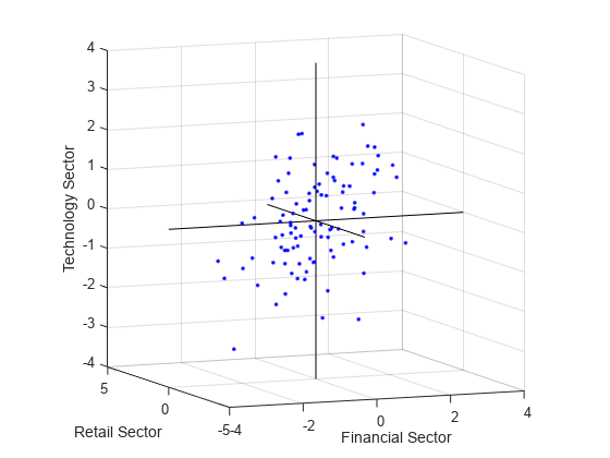
Sometimes, it is useful to be able to classify an observation based on its factor scores. For example, if you accepted the three-factor model and the interpretation of the rotated factors, you might want to categorize each week in terms of how favorable it was for each of the three stock sectors, based on the data from the 10 observed stocks. Because the data in this example are the raw stock price changes, and not just their correlation matrix, you can have factoran return estimates of the value of each of the three rotated common factors for each week. You can then plot the estimated scores to see how the different stock sectors were affected during each week.

[LoadingsPM,specVarPM,TPM,stats,F] = factoran(stocks, 3,'rotate','promax');

plot3(F(:,1),F(:,2),F(:,3),'b.')
line([-4 4 NaN 0 0 NaN 0 0], [0 0 NaN -4 4 NaN 0 0],[0 0 NaN 0 0 NaN -4 4], 'Color','black')
xlabel('Financial Sector')
ylabel('Retail Sector')
zlabel('Technology Sector')
grid on
axis square
view(-22.5, 8)

Oblique rotation often creates factors that are correlated. This plot shows some evidence of correlation between the first and third factors, and you can investigate further by computing the estimated factor correlation matrix.

inv(TPM'*TPM);

Visualize the Results

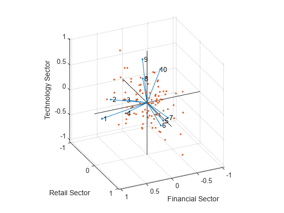
You can use the biplot function to help visualize both the factor loadings for each variable and the factor scores for each observation in a single plot. For example, the following command plots the results from the factor analysis on the stock data and labels each of the 10 stocks.

biplot(LoadingsPM,'scores',F,'varlabels',num2str((1:10)'))
xlabel('Financial Sector')
ylabel('Retail Sector')
zlabel('Technology Sector')
axis square
view(155,27)

In this case, the factor analysis includes three factors, and so the biplot is three-dimensional. Each of the 10 stocks is represented in this plot by a vector, and the direction and length of the vector indicates how each stock depends on the underlying factors. For example, you have seen that after promax rotation, the first four stocks have positive loadings on the first factor, and unimportant loadings on the other two factors. That first factor, interpreted as a financial sector effect, is represented in this biplot as one of the horizontal axes. The dependence of those four stocks on that factor corresponds to the four vectors directed approximately along that axis. Similarly, the dependence of stocks 5, 6, and 7 primarily on the second factor, interpreted as a retail sector effect, is represented by vectors directed approximately along that axis.

Each of the 100 observations is represented in this plot by a point, and their locations indicate the score of each observation for the three factors. For example, points near the top of this plot have the highest scores for the technology sector factor. The points are scaled to fit within the unit square, so only their relative locations can be determined from the plot.

You can use the Data Cursor tool from the Tools menu in the figure window to identify the items in this plot. By clicking a stock (vector), you can read off that stock's loadings for each factor. By clicking an observation (point), you can read off that observation's scores for each factor.