Evaluate Optimal Number of Clusters
Identify the optimal number of clusters in a data set by using the evalclusters function.
As an alternative, you can interactively perform k-means clustering by using the Cluster Data Live Editor task.
Load the fisheriris data set.
load fisheriris
X = meas;
y = categorical(species);
X is a numeric matrix that contains two sepal and two petal measurements for 150 irises. y is a cell array of character vectors that contains the corresponding iris species.
Evaluate the optimal number of clusters from 1 to 10 using the Calinski-Harabasz criterion. Cluster the data using the k-means clustering algorithm.
evaluation = evalclusters(X,"kmeans","CalinskiHarabasz",KList=1:10)
evaluation =
  CalinskiHarabaszEvaluation with properties:

    NumObservations: 150
         InspectedK: [1 2 3 4 5 6 7 8 9 10]
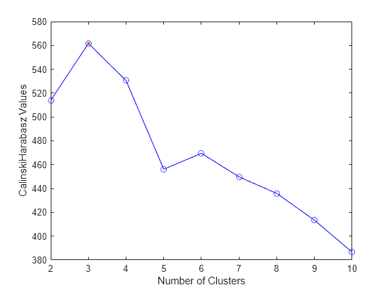
    CriterionValues: [NaN 513.9245 561.6278 530.4871 456.1279 469.5068 449.6410 435.8182 413.3837 386.5571]
           OptimalK: 3


  Properties, Methods
The OptimalK value indicates that, based on the Calinski-Harabasz criterion, the optimal number of clusters is 3.
Visualize the cluster evaluation results for each number of clusters.
plot(evaluation)
legend(["Criterion values","Criterion value at OptimalK"])

Most clustering algorithms require prior knowledge of the number of clusters. When the number of clusters is not known, use cluster evaluation techniques to determine the number of clusters present in the data based on a specified metric.
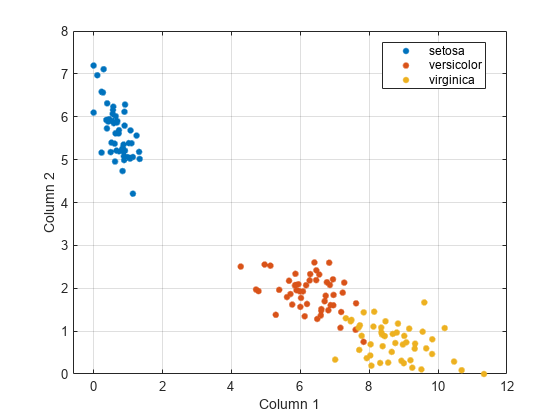
Note that identifying three clusters in the data is consistent with having three species in the data.
categories(y)
ans = 3×1 cell
    {'setosa'    }
    {'versicolor'}
    {'virginica' }
To visualize the data, compute a nonnegative rank-2 approximation of the data.
reducedX = nnmf(X,2);
The original features are reduced to two features. Because none of the features are negative, nnmf guarantees that the features are nonnegative.
Visualize the three clusters using a scatter plot. Use color to indicate the iris species.
gscatter(reducedX(:,1),reducedX(:,2),y)
xlabel("Column 1")
ylabel("Column 2")
grid on

See Also
evalclusters | nnmf | gscatter | Cluster
Data