Ensemble Regularization

Regularization is a process of choosing fewer weak learners for an ensemble in a way that does not diminish predictive performance. Currently you can regularize regression ensembles. (You can also regularize a discriminant analysis classifier in a non-ensemble context; see Regularize Discriminant Analysis Classifier.)

The regularize method finds an optimal set of learner weights α_t that minimize

$\sum_{n = 1}^{N} w_{n} g ((\sum_{t = 1}^{T} α_{t} h_{t} (x_{n})), y_{n}) + λ \sum_{t = 1}^{T} | α_{t} | .$

Here

λ ≥ 0 is a parameter you provide, called the lasso parameter.
h_t is a weak learner in the ensemble trained on N observations with predictors x_n, responses y_n, and weights w_n.
g(f,y) = (f – y)² is the squared error.

The ensemble is regularized on the same (x_n,y_n,w_n) data used for training, so

$\sum_{n = 1}^{N} w_{n} g ((\sum_{t = 1}^{T} α_{t} h_{t} (x_{n})), y_{n})$

is the ensemble resubstitution error. The error is measured by mean squared error (MSE).

If you use λ = 0, regularize finds the weak learner weights by minimizing the resubstitution MSE. Ensembles tend to overtrain. In other words, the resubstitution error is typically smaller than the true generalization error. By making the resubstitution error even smaller, you are likely to make the ensemble accuracy worse instead of improving it. On the other hand, positive values of λ push the magnitude of the α_t coefficients to 0. This often improves the generalization error. Of course, if you choose λ too large, all the optimal coefficients are 0, and the ensemble does not have any accuracy. Usually you can find an optimal range for λ in which the accuracy of the regularized ensemble is better or comparable to that of the full ensemble without regularization.

A nice feature of lasso regularization is its ability to drive the optimized coefficients precisely to 0. If a learner's weight α_t is 0, this learner can be excluded from the regularized ensemble. In the end, you get an ensemble with improved accuracy and fewer learners.

Regularize a Regression Ensemble

Open Live Script

This example uses data for predicting the insurance risk of a car based on its many attributes.

Load the imports-85 data into the MATLAB® workspace.

load imports-85;

Look at a description of the data to find the categorical variables and predictor names.

Description

Description = 9x79 char array
    '1985 Auto Imports Database from the UCI repository                             '
    'http://archive.ics.uci.edu/ml/machine-learning-databases/autos/imports-85.names'
    'Variables have been reordered to place variables with numeric values (referred '
    'to as "continuous" on the UCI site) to the left and categorical values to the  '
    'right. Specifically, variables 1:16 are: symboling, normalized-losses,         '
    'wheel-base, length, width, height, curb-weight, engine-size, bore, stroke,     '
    'compression-ratio, horsepower, peak-rpm, city-mpg, highway-mpg, and price.     '
    'Variables 17:26 are: make, fuel-type, aspiration, num-of-doors, body-style,    '
    'drive-wheels, engine-location, engine-type, num-of-cylinders, and fuel-system. '

The objective of this process is to predict the "symboling," the first variable in the data, from the other predictors. "symboling" is an integer from -3 (good insurance risk) to 3 (poor insurance risk). You could use a classification ensemble to predict this risk instead of a regression ensemble. When you have a choice between regression and classification, you should try regression first.

Prepare the data for ensemble fitting.

Y = X(:,1);
X(:,1) = [];
VarNames = {'normalized-losses' 'wheel-base' 'length' 'width' 'height' ...
  'curb-weight' 'engine-size' 'bore' 'stroke' 'compression-ratio' ...
  'horsepower' 'peak-rpm' 'city-mpg' 'highway-mpg' 'price' 'make' ...
  'fuel-type' 'aspiration' 'num-of-doors' 'body-style' 'drive-wheels' ...
  'engine-location' 'engine-type' 'num-of-cylinders' 'fuel-system'};
catidx = 16:25; % indices of categorical predictors

Create a regression ensemble from the data using 300 trees.

ls = fitrensemble(X,Y,'Method','LSBoost','NumLearningCycles',300, ...
    'LearnRate',0.1,'PredictorNames',VarNames, ...
    'ResponseName','Symboling','CategoricalPredictors',catidx)

ls = 
  RegressionEnsemble
           PredictorNames: {1x25 cell}
             ResponseName: 'Symboling'
    CategoricalPredictors: [16 17 18 19 20 21 22 23 24 25]
        ResponseTransform: 'none'
          NumObservations: 205
               NumTrained: 300
                   Method: 'LSBoost'
             LearnerNames: {'Tree'}
     ReasonForTermination: 'Terminated normally after completing the requested number of training cycles.'
                  FitInfo: [300x1 double]
       FitInfoDescription: {2x1 cell}
           Regularization: []

The final line, Regularization, is empty ([]). To regularize the ensemble, you have to use the regularize method.

cv = crossval(ls,'KFold',5);
figure;
plot(kfoldLoss(cv,'Mode','Cumulative'));
xlabel('Number of trees');
ylabel('Cross-validated MSE');
ylim([0.2,2])

Figure contains an axes object. The axes object with xlabel Number of trees, ylabel Cross-validated MSE contains an object of type line.

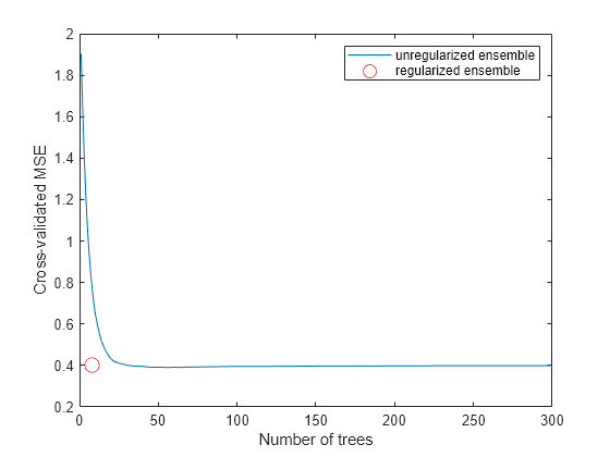
It appears you might obtain satisfactory performance from a smaller ensemble, perhaps one containing from 50 to 100 trees.

Call the regularize method to try to find trees that you can remove from the ensemble. By default, regularize examines 10 values of the lasso (Lambda) parameter spaced exponentially.

ls = regularize(ls)

ls = 
  RegressionEnsemble
           PredictorNames: {1x25 cell}
             ResponseName: 'Symboling'
    CategoricalPredictors: [16 17 18 19 20 21 22 23 24 25]
        ResponseTransform: 'none'
          NumObservations: 205
               NumTrained: 300
                   Method: 'LSBoost'
             LearnerNames: {'Tree'}
     ReasonForTermination: 'Terminated normally after completing the requested number of training cycles.'
                  FitInfo: [300x1 double]
       FitInfoDescription: {2x1 cell}
           Regularization: [1x1 struct]

The Regularization property is no longer empty.

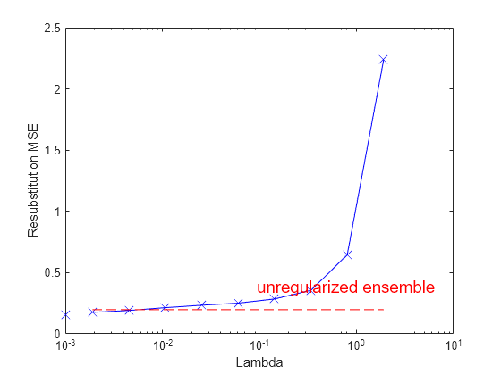
Plot the resubstitution mean-squared error (MSE) and number of learners with nonzero weights against the lasso parameter. Separately plot the value at Lambda = 0. Use a logarithmic scale because the values of Lambda are exponentially spaced.

figure;
semilogx(ls.Regularization.Lambda,ls.Regularization.ResubstitutionMSE, ...
    'bx-','Markersize',10);
line([1e-3 1e-3],[ls.Regularization.ResubstitutionMSE(1) ...
     ls.Regularization.ResubstitutionMSE(1)],...
    'Marker','x','Markersize',10,'Color','b');
r0 = resubLoss(ls);
line([ls.Regularization.Lambda(2) ls.Regularization.Lambda(end)],...
     [r0 r0],'Color','r','LineStyle','--');
xlabel('Lambda');
ylabel('Resubstitution MSE');
annotation('textbox',[0.5 0.22 0.5 0.05],'String','unregularized ensemble', ...
    'Color','r','FontSize',14,'LineStyle','none');

Figure contains an axes object. The axes object with xlabel Lambda, ylabel Resubstitution MSE contains 3 objects of type line.

figure;
loglog(ls.Regularization.Lambda,sum(ls.Regularization.TrainedWeights>0,1));
line([1e-3 1e-3],...
    [sum(ls.Regularization.TrainedWeights(:,1)>0) ...
    sum(ls.Regularization.TrainedWeights(:,1)>0)],...
    'marker','x','markersize',10,'color','b');
line([ls.Regularization.Lambda(2) ls.Regularization.Lambda(end)],...
    [ls.NTrained ls.NTrained],...
    'color','r','LineStyle','--');
xlabel('Lambda');
ylabel('Number of learners');
annotation('textbox',[0.3 0.8 0.5 0.05],'String','unregularized ensemble',...
    'color','r','FontSize',14,'LineStyle','none');

Figure contains an axes object. The axes object with xlabel Lambda, ylabel Number of learners contains 3 objects of type line.

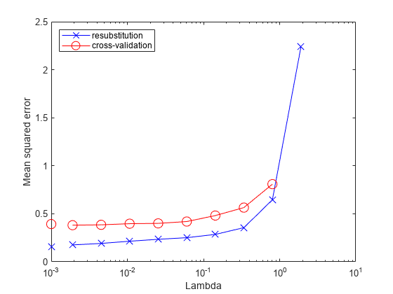
The resubstitution MSE values are likely to be overly optimistic. To obtain more reliable estimates of the error associated with various values of Lambda, cross validate the ensemble using cvshrink. Plot the resulting cross-validation loss (MSE) and number of learners against Lambda.

rng(0,'Twister') % for reproducibility
[mse,nlearn] = cvshrink(ls,'Lambda',ls.Regularization.Lambda,'KFold',5);

Warning: Some folds do not have any trained weak learners.

figure;
semilogx(ls.Regularization.Lambda,ls.Regularization.ResubstitutionMSE, ...
    'bx-','Markersize',10);
hold on;
semilogx(ls.Regularization.Lambda,mse,'ro-','Markersize',10);
hold off;
xlabel('Lambda');
ylabel('Mean squared error');
legend('resubstitution','cross-validation','Location','NW');
line([1e-3 1e-3],[ls.Regularization.ResubstitutionMSE(1) ...
     ls.Regularization.ResubstitutionMSE(1)],...
    'Marker','x','Markersize',10,'Color','b','HandleVisibility','off');
line([1e-3 1e-3],[mse(1) mse(1)],'Marker','o',...
    'Markersize',10,'Color','r','LineStyle','--','HandleVisibility','off');

Figure contains an axes object. The axes object with xlabel Lambda, ylabel Mean squared error contains 2 objects of type line. These objects represent resubstitution, cross-validation.

figure;
loglog(ls.Regularization.Lambda,sum(ls.Regularization.TrainedWeights>0,1));
hold;

Current plot held

loglog(ls.Regularization.Lambda,nlearn,'r--');
hold off;
xlabel('Lambda');
ylabel('Number of learners');
legend('resubstitution','cross-validation','Location','NE');
line([1e-3 1e-3],...
    [sum(ls.Regularization.TrainedWeights(:,1)>0) ...
    sum(ls.Regularization.TrainedWeights(:,1)>0)],...
    'Marker','x','Markersize',10,'Color','b','HandleVisibility','off');
line([1e-3 1e-3],[nlearn(1) nlearn(1)],'marker','o',...
    'Markersize',10,'Color','r','LineStyle','--','HandleVisibility','off');

Figure contains an axes object. The axes object with xlabel Lambda, ylabel Number of learners contains 2 objects of type line. These objects represent resubstitution, cross-validation.

Examining the cross-validated error shows that the cross-validation MSE is almost flat for Lambda up to a bit over 1e-2.

Examine ls.Regularization.Lambda to find the highest value that gives MSE in the flat region (up to a bit over 1e-2).

jj = 1:length(ls.Regularization.Lambda);
[jj;ls.Regularization.Lambda]

ans = 2×10

    1.0000    2.0000    3.0000    4.0000    5.0000    6.0000    7.0000    8.0000    9.0000   10.0000
         0    0.0019    0.0045    0.0107    0.0254    0.0602    0.1428    0.3387    0.8033    1.9048

Element 5 of ls.Regularization.Lambda has value 0.0254, the largest in the flat range.

Reduce the ensemble size using the shrink method. shrink returns a compact ensemble with no training data. The generalization error for the new compact ensemble was already estimated by cross validation in mse(5).

cmp = shrink(ls,'weightcolumn',5)

cmp = 
  CompactRegressionEnsemble
           PredictorNames: {1x25 cell}
             ResponseName: 'Symboling'
    CategoricalPredictors: [16 17 18 19 20 21 22 23 24 25]
        ResponseTransform: 'none'
               NumTrained: 8

The number of trees in the new ensemble has notably reduced from the 300 in ls.

Compare the sizes of the ensembles.

sz(1) = whos('cmp'); sz(2) = whos('ls');
[sz(1).bytes sz(2).bytes]

ans = 1×2

       96476     3390154

The size of the reduced ensemble is a fraction of the size of the original. Note that your ensemble sizes can vary depending on your operating system.

Compare the MSE of the reduced ensemble to that of the original ensemble.

figure;
plot(kfoldLoss(cv,'mode','cumulative'));
hold on
plot(cmp.NTrained,mse(5),'ro','MarkerSize',10);
xlabel('Number of trees');
ylabel('Cross-validated MSE');
legend('unregularized ensemble','regularized ensemble',...
    'Location','NE');
hold off

Figure contains an axes object. The axes object with xlabel Number of trees, ylabel Cross-validated MSE contains 2 objects of type line. One or more of the lines displays its values using only markers These objects represent unregularized ensemble, regularized ensemble.

The reduced ensemble gives low loss while using many fewer trees.

Ensemble Regularization

Regularize a Regression Ensemble

See Also

Related Topics